"Master and Slave" fluidic amplifier cascade

“MASTER AND SLAVE" FLUIDIC AMPLIFIER CASCADE

Václav TESAx

Abstract: No-moving-part fluidics recently found interesting application in generation of gas microbubbles by oscillating the inlet flow of the gas into the aerator. The oscillation frequency has to be high and this calls for small size of the oscillator. On the other hand, most microbubble applications require a large total gas flow. This calls for large fluidic device – a les expensive alternative than “numbering up” (several oscillators in parallel). The contradiction of the large and small scale is solved by the “MASTER & SLAVE” fluidic circuit: large output device controlled by a small oscillator. Paper discusses basic problems encountered in designing the circuit which requires matching the characteristics of the two devices.

1. I

NTRODUCTION

The problem discussed in this paper arose in application of no-moving-part fluidics to generation of very small gas bubbles in liquids [1]. The microbubbles bring considerable improvement in many promising applications, from waste water processing [1], growing monocellular plants [2] (used as the starting step of a food chain [3], for production of biodiesel [4], or for carbon dioxide sequestration [5]) up to flotation separation of proteins and other substances and objects [6]. The benefit brought by microbubbles is mainly the large total mass transfer surface together with slow rising velocity of the bubbles in the liquid. This ensures a large and long-lasting gas transfer interface. Traditional steady flow aerators – with however small gas exit orifices - cannot produce the microbubbles due to the instability of bubble formation caused by the very fundamental Young-Laplace law (e.g., [7]). Fluidics made possible a simple and attractive solution [1, 2]. Flow pulsation is generated in the gas inlet by a simple no-moving-part fluidic oscillator – essentially nothing more than just a special shaping the inlet geometry – and causes fragmentation of the bubbles at the aerator exits.

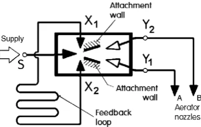
In principle, the fluidic oscillators consist of two parts (Fig. 1) – a no-moving-part amplifier, usually a bistable one based on the Coanda effect (Fig. 2), and a feedback loop channel. Several alternative ways of the feedback arrangement are known. Because of its simplicity, the Spyropoulos type feedback (discussed in detail in [8]), as presented schematically in Fig. 1, with just a single channel connecting the two control terminals of the amplifier, was the preferred layout in the tests performed by this author so far [9].

Efficiency of the fluidic oscillator in its bubble fragmentation role was found to increase with increasing oscillation frequency. This calls for a small oscillator for several reasons:

x _{Institute of Thermomechanics v.v.i., Academy of Sciences of the Czech Republic, 182 00 Prahe 8,}

Dolejškova 5, Czech Republic EPJ Web of Conferences , 010 (2012) DOI: 10.1051/epjconf/201225010

© Owned by the authors, published by EDP Sciences, 2012

Figure 1: Schematic representation of the fluidic oscillator with the single feedback loop, connecting the control terminals X1 and X2 , used by the author in the applications. The black triangles are representations of nozzles (cross section decreasing in the flow direction), white triangles represent diffusers.

a) the frequency increases with shorter propagation time of the switching signal in the feedback loop, which therefore has to be short. It cannot be decreased below certain limits if the fluidic amplifier is not correspondingly small.

b) a significant role among the factors that determine the frequency plays the switching time of the amplifier. This correlates with the time-of-flight of the fluid - between the supply nozzle exit and the collector entrance. Obviously, this time is also longer in a larger amplifier.

On the other hand, many of the applications named above call for generating the bubbles in large quantities. Growing the algae for biodiesel production or carbon sequestration from smokestacks requires large scale of the operation. One possibility how to handle the corresponding large gas throughput is, of course, the “numbering-up” (e.g., [10]) – operating a large number of the oscillators in parallel. Generally more economical is keeping the oscillator number small and having them very large. This, of course, contradicts the above listed items (a) and (b).

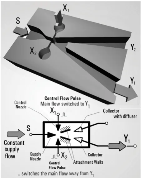
Figure 2: An example of an unvented Coanda-effect bistable amplifier and (bottom) its schematic representation (cf. Fig. 1). The constant fluid flow supplied into S forms in the supply nozzle a jet that attaches with equal probability to one of the two attachment walls. Each wall leads it into one of the two outputs. Even a small control flow pulse switches it onto the opposite attachment wall and thereby to the other output terminal.

compressed air (not to speak those applications handling more valuable fluids). The amplifiers have to be invented, as shown in Fig. 2. This means the properties of the two stages have to be closely matched. The matching is, in general, much more difficult than the between the well-known analogous situation in the case of electronic amplifiers. First, the amplifier stages in fluidics have unpleasantly larger number of the terminals (note the five terminals

S, X

1,

X

2,

Y

1, and

Y

2in Fig. 2). Note in Fig. that there are two output terminals in the “MASTER” to be matched simultaneously with the two input terminals of the “Slave”. In fact, the conditions (pressure and flow rate) in each of the five terminals in Fig. 2 influence the state in every of the remaining four terminals. Second complicating factor is the non-linearity of the properties.

2. C

HARACTERISTICS

Beacuse of the large number of variables and nonlinearity, it is not effective to describe the properties of fluidic amplifiers by formulas. It became customary to present them in diagrammatic form, as families of curves called characteristics. Theoretically, the number of the curves in each family is infiite. It is usually necessary to limit the number of them by considering to a certain range of the variables and by selecting a certain resonable step

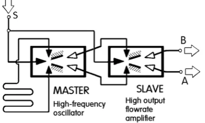
Figure 3:Representation of the fluidic circuit with two amplifiers, as it was used in early tests of MASTER & SLAVE configuration. It solves the contradictory size problem encountered in microbubble aeration: high oscillation frequency calling for small size of the oscillator together with high gas throughput which, of course, calls for a large size.

Figure 4:Schematic representation of the MASTER & SLAVE oscillator, using the symbols for the fluidic element and their components as they are presented above in Fig. 2. For simplicity, both amplifiers are supplied (as they did in Fig. 3) with the air at the same pressure.

between the parameter values. To limit the number of the curve families, some of them are removed from the considerations by an assumption of constancy of some of the variables.

Figure 5: A typical planar fluidic bistable amplifier (dimensions in millimetres). Geometry of its core part was used by the author in many of his applications of fluidics. It is essentially the geometry [A] stemming from al long time ago as 1975, ref. [12]. In some later versions the control nozzle width was increased from the small 0.35 b (i.e. 0.5 mm) shown here.

to which the conditions in other terminal are presented - is the _OFF output terminal Y2. An important fact, utilised in Figs. 7 and 8, is similarity (usually only approximate) of the curves in a particular 'e = f (oM) family at different supply flow rates (which are characterised by the Reynolds number evaluated for the supply nozzle exit conditions). This property – called Eulerian similarity – may be used to simplify the presentation. If the Eulerian similarity were perfect, all curves of a particuar family could be squeezed into just a single universal curve by plotting it in dimensionless, relative co-ordinates.

Figure 6: Definition of the quantities used in plotting of the output characteristics presented in Fig. 7. For simplicity, both control flow rates are considered zero – a regime well corresponding to the switching of the amplifier by short control pulses, although unfortunately not the regimes in the “MASTER & SLAVE” circuit.

The example in Fig. 7 shows there in real situations are some Reynolds number dependence effects, but these are usually not substantial (especially if the Reynolds number values are large) so that the simplification obtained by presentation in the dimensionless quantities is very useful.

The schematic representation in Fig. 6 shows the evaluated variables in setting up the output characteristics of a bistable amplifier. In many applications such amplifiers are switched between their two stable regimes by applying only a brief flow pulse into tone of the control inlets – so that for the rest of the time the flows in the control inlets are zero. This is the reason behind, as indicated in Fig. 6, the simplification of the output characterstics by assuming blocked control terminals. There are then only two variable

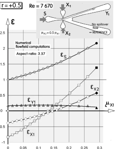
Figure 8: Dimensionless input characteristics of the author’s amplifier from Fig. 5. Result of numerical computations with two-equation model of turbulence for the no-spillover condition and opposing flow in the control terminal X2, the magnitude of which was kept at one half of the main flow in X1. ;

flow rates, the output mass flow rate oMY1 [kg/s] in the _ON terminal and the supply mass flow rate oMS [kg/s]. The latter is in many practical uses constant, so that the relatuve output flow rate in the role of the independent variable (Fig. 7) is

... (1)

The analogous independent variable in the control characteristic presented in Fig. 8 is

... (2)

The vertical co-ordinate in both Fig. 7 and Fig. 8 is essentially the specific energy difference 'e, consisting of the sum of specific pressure energy difference and the difference in specific kinetic energy [11], non-dimensonalised by being related to the supply specific energy difference. An important regime in Fig. 7 is the no-spillover state

... (3)

with all the supplied flow leaving through the ON output terminal Y1 . Because he specific energy difference 'eS between the supply terminal S and the reference terminal Y2 actually varies somewhat when the independent variable eq. (1) varies, the exact definition of the variable plotted on the vertical axes in Figs. 7 and 8 is

... (4)

The geometry of the amplifiers discussed here – the geometry [A] - was very successful in having achieved pressure recovery ~60 % in the no-spillover states – and even higher ~70 % if some small part of the flow was allowed to spill into the OFF output (reference) terminal Y2. These regimes were arrived at bu partiaql blockage of the flow through the ON output. The Coanda effect – as well as the internal feedback obtained by the bi-cuspid splitter – maintaned in such blockage the main jet at the ON attachment wall. If, however, the blockage effect was increased, the flow is seen in Fig. & to stall and finally separated and load-switch into the terminal Y2.

In the case of the input characteristics, Fig. 8, the assumption of blocked control terminals applied in Fig. 7 is, of course, not acceptable. The independent variable eq. (2) is evaluated from the control flow in the ON side terminal X1, but also the flow in the other OFF side terminal X2 may be non-zero. To limit somewhat the amount of evaluated variables, an assumption applied was the flow at the OFF side is related to the independent variable control flow by constancy of the parameter

... (5) The example of the control characteristics in Fig. 8 was actually computed (by numerical flowfield solutions) for the constanmt value r = + 0.5. Of the curves there, the most important from the point of view of circuit slutions discussed here are the two ones that

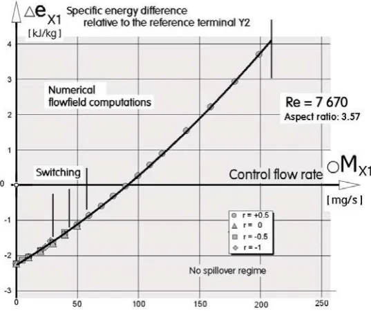
Figure 10: Computed behaviour of the X1 (main, ON-side) input at different constant values of the control flow ratio r. All four plotted curves coincide into effectively a single line that reflects the quadratic increase of the pressure loss in the narrow control nozzle.

characterise the conditions in the control terminals X1 and X2. They are plotted alone in the two subsequent illustrations, Figs. 9 and 10, for four different constant values of the parameter r. The control nozzles in the amplifier presented in Fig. 5, for which all these computations were performed, are very narrow compared with what is a standard in fluidics. The reason for this choice was the particular situation when geometry [A] was designed: the amplifier was then rather large and worked with large air flows at low pressure levels while the available air for the control actions was in limited flow rates but at almost unlimited pressure levels. The small control nozzles thus generate very intensive narrow jets that, despite the small flow rate can switch effectively the main flow. The fact that there were relative large pressure differences across the control nozzles was of no importance.

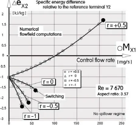
This character of the control nozzles is reflected in the curves plotted in the Figs. 9 and 10. The specific energy drops 'eX1 and 'eX2 are little influenced by the aerodynamic processes inside the interaction cavity of the amplifier, the behaviour is mainly dictated by the pressure drops across the control nozzles. In Fig. 9, the basic behaviour is the one for r = 0, i.e. zero flow in the control terminal X2. If the flow in the control terminal X2 is positive (out from the nozzle into the interaction cavity), the specific energy 'eX2 increases with increasing control flow. On the other hand, if there is at negative r a suction into the control terminal X2, the corresponding specific energy 'eX2 quite rapidly decreases with increasing control flow. In Fig. 10, the practical absence of the influence of the aerodynamic processes inside the interaction cavity is even more apparent. The four curves for different values r indicate practically the same

Figure 11: The steady-state regime matching of the MASTER and SLAVE devices. The task is to find how the flow rate bifurcates into the two flow paths that connect the two amplifiers and whether the resultant flow into the SLAVE device suffices for the switching.

specific energy 'eX1 increase with increasing control flow. This increase is obviously just the effect of the pressure drop across the narrow control nozzle.

3. C

HARACTERISTICS FOR THE

M

&

S

CIRCUIT

The increase of the number of variables brought into the problem by the second amplifier makes the analysis more difficult – even if it is accepted, for simplification, to neglect the difficulties associated with the dynamics of switching in the SLAVE amplifier. The attentian concentrates here only on the conditions before (Fig. 11) and after (Fig. 13) the switching. Also, it is assumed that the conditions may be evaluated by applying the characteristics that were evaluated for the steady flow regimes.

This quasi-steady approach to the analysis of the conditions is base upon the ideas presented in Fig. 12. The output characteristics of the MASTER amplifier are compared with the input characteristics of the SLAVE device. The comparison then makes it possible to obtain the information whether or not the MASTER output flows siffice for the switching that should take place in the SLAVE.

As the first step in this analysis, let us consider the circuit consisting at bot the MASTER and SLAVE stage by the same amplifiers. Speaking here about amplifiers means that the conditions for achieving the switching state are favourable – in an amplifier, the ouput flows are significantly stronger than the input flows needed for the switching. Then in ther next step, the analysis should provide an answer to the question how much may be the downstream amplifier, SLAVE, scaled up still retaining its chapability to be switched.

Figure 12: The basic ideas of the steady-state regime matching: the answers sought are obtained by comparison of the MASTER output and SLAVE input characteristics. In the SLAVE case, the usual reference R1 is inconvenient, the characteristics are to be transformed for the reference in R2.

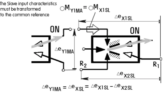
characteristicvs require being related top the same reference. The input characteristics of the SLAVE amplifier have to be transformed by using instead of the traditional reference R1 (Fig. 12) the reference R2 in the OFF-side control line.

The other transformation that has to be made to the characteristics in an approach based on the idea of size scaling is the necessity to work with absolute rather than the relative dimensionless variables. In the example to be discussed, the characteristics – presented in Figs. 14 (MASTER output) and 15 (SLAVE input), were transformed to the same value of the supply flow rate, corresponding to sypply nozzle exit Reynolds number Re = 7 670. The loading curve plotted in Fig. 14 was evaluated from the dimensionless curve in Fig. 7. Only its stable part, not influenced by the stalling, is actually used. The sumbols placed on the curve in Fig. 14 show the values of the flow ratio parameter r. It is evident that the useful part of the loading curve corresoponds to the values from r = - 0.5 to r = 0 or even less – to transfer hydraulic

Figure 13: The same idea of the steady-state regime matching may be used for checking the conditions after the SLAVE flow is switched. This is, however, rarely done.

Figure 14: The loading curve of the MASTER amplifier from Fig 7, here re-computed into absolute values of the variables for a particular constant supply flow rate.

Figure 15: Input characteristics of the amplifier shown in Fig. 5 re-computed for the common reference in the MASTER & SLAVE circuit (cf. Fig. 11) as the difference between the curves of Fig. 9 and 10. Considering the achievable values in the MASTER amplifier, only the cases r = 0 and r = -0.5 are of interest here.

Correspondingly, of the four curves r = const, as shown e.g. in Fig. 9, the region of interest in the transformed input characteristics presente in Fig. 15 will be only between the curves for r = - 0.5 to r = 0.

4. L

OGARTHMIC SCALES

The scaling of fluidic devices in the procedure of matching the MASTER and SLAVE would call for a regression step from the introduction of the universal dimensionless plotting of the characteristics discussed in the section 2 above. The graphical procedure of superimposing the output and input characteristics would necessitate plotting separately the curves in a family (for suitable size steps between the members of the family). The laws governing the re-plotting may be usefully presented by considering the expression for the quadratic dissipance Q [m2_/kg2_{] defined as [11, 13]}

... (6)

- this may be re-written into

... (7) where cD is the dimensonless drag (or loss) coefficient, dependent on Reynolds number, v [m3/kg] is the specific volume of the gas, and F [m2] is the cross-section area.

The family of characteristics of a family of constant size (F = const) fluidic devices supplied by different flow rates of the gas is re-drawn following the law

... (8) In the present case, the interest is mainly in the families of geometrically similar devices

Figure 16: The advantage obtained by re-plotting the characteristic in the logarithmic scales (cf. Fig. 18). Due to the Eulerian similarity (coincidence of lines at various supply flows in Fig. 7) the behaviour of an amplifier at various supply flow and pressure conditions is found by simple shifting of the logarithmic plot along the line of constant dissipance Q.

Figure 17: Another use of the logarithmic-scales plotting of characteristics: the behaviour of varying the size of geometrically similar amplifiers is found by simple shifting of the logarithmic plot along the flow rate axis. No Reynolds number effects are assumed.

of various sizes. Everything else ( the fluid as well as the supply pressure – and hence 'eS) the law for drawing the family is

... (9) and hence the flow rate proportional to the square of the increasing length scale

l

... (10) A way how to circumvent the rather laborious re-drawing of characteristics was suggested in 1971 by Dr. Tippetts at the University of Sheffield, U.K.. According to his proposal, the characteristics are plotted in logarithmic scales – preferably on a

Figure 19: The input curves of the SLAVE amplifier from Fig 15 are here plotted in the logarithmic scales. The dot symbols at the end of r = 0 and r = -0.5 lines indicate the conditions at which the amplifier is switched. The arrows show the usual progress of the increasing flow rate before this happens.

transparent sheet. Instead of actually plotting the family, the logarithmic diagram is thenshifted over the plotting area. Figure 16 shows the shifting of the logarithmic diagram following the law eq. (8) while the next Fig. 17 shows the sfigting following the law eq.(10).

Logarithmic presentation of the loading characteristics from Fig. 14 is here shown in Fig. 18 and the input characteristics from Fig. 15 (leaving the practically unattainable values of the flow ratio r) is shown in Fig. 19. The next Fig. 20 then shows superposition of these input and output characteristics. Switching of the SLAVE amplifier is possible of the round sumbils at the ends of the input lines are in the shaded arera to the left of the loading curve. As might be expected, in the case of two equal amplifiers there is no problem with the switching.

5. M

ATCHING PROCEDURE

The conclusion arrived at in the previous section is, of course, not surprising. The same procedure may be, of course, applied to a different pair of fluidic amplifiers, once their characteristics are known. What the procedure discussed here is actually after is the more demanding task of finding the scaling law that governs increasing the size of geometrically similar SLAVE amplifiers while maintaining their capability of being switched by the MASTER upstream.

It may be quite desirable to get the switching in the no-spillover regime. The attention is therefore concentrated on only the r = 0 curve from Fig. 20. This will be shifted in the logarithmic co-ordinates following the law eq.(10) as the SLAVE amplified is

Figure 20: As expected on an amplifier, the computed input characteristics from Figs. 18 and 19 of the same device in both MASTER and SLAVE roles at the same supply flow conditions are safely at the left-hand side from the experimentally measured output characteristics.

scaled up. As seen in Fig. 21, it would be quite safe to increase the SLAVE to twice its original length scale size with the switching point retained safely in the shaded area of Fig. 20. What is more, even increasing the linear dimensions to three times the original values does not endanger the switching. This, however, is not the case with increase to 5-times or 10-times the original size. In addition, the illustration also shows, that it is possible to obtain the switching exactly in the no spillover regime of the SL:AVE amplifier, scaled slightly less than to three times it original size, is operated with the increased supply gas pressure. Such a close matching may be dangerous, of course, especially as the discussed approach neglects the dynamics of the switching – the SLAVE is then in danger of missing some of the switching signals from the opscillating MASTER.

6. C

ONCLUSIONS

Figure 21: The scaling up of the amplifier from Fig. 5 to two- or three-times larger linear dimensions still retains the controllability. The would cease to be the case after increasing the size five or ten times. An amplifier scale slightly less than three times and supplied by increased supply pressure may bring the switching conditions to the ideal no-spillover state.

7. R

EFERENCES

[1] Zimmerman, W. B., Tesa, V.: “Bubble Generation for Aeration and Other Purposes”, European Patent Nr. 07824345, filed Oct. 2007 granted May 2011

[2] Zimmerman, W. B., Hewakandamby B. N., Tesa V., Bandulasena H.C.H., Omotowa O. A.: „On the Design and Simulation of an Airlift Loop Bioreactor with Microbubble Generation by Fluidic Oscillation“, Food and Bioproducts Processing, Vol. 97, doi:10.1016/j.fbp.2009.03.006, p. 215, 2009

[3] Gao K.: "Chinese studies on the edible blue-green alga, Nostoc flagelliforme: A review", Journal of Applied Phycology, Vol. 10, p. 37, 1998

[4] Demirbas M.F.: “Biofuels from algae for sustainable development”, Applied Energy, Vol. 88, p.3473, 2011

[5] Shi B., Wideman G., Wang J.H.: “A New Approach of BioCO2 Fixation by Thermoplastic Processing of Microalgae”, Journal of Polymers and the Environment, in Press, 2011-10-25

[6] Teixeira M. R., Rosa M. J.: "Comparing dissolved air flotation and conventional sedimentation to remove cyanobacterial cells of Microcystis aeruginosa Part 1: The key operating conditions", Separation and Purification Technology, Vol. 52, p. 84, 2006

[7] Finn R.: "Equilibrium Capillary Surfaces", Springer-Verlag, New York, 1986

[8] Tippetts J.R., Ng H.K., Royle J.K.: "An oscillating bistable fluid amplifier for use as a flowmeter", Fluidics Quarterly, Vol. 5, p. 28, 1973

[9] Tesa V., Hung C.-H., Zimmerman W. B.: “No-Moving-Part Hybrid-Synthetic Jet Actuator“, Sensors and Actuators A, Vol. 125, p. 159, 2006

[10] Tesa V.: “Bifurcating Channels Supplying ‘Numebred-Up’ Microreactors”, Chemical Engineering Research and Design, in Press, 2011

[11] Chapter Tesa V.: “Characterization of two-terminal devices", pp. 223-253 in the monograph " _{Microfluidics: History, Theory, and Applications",} Ed. W. B. J. Zimmerman, CISM Courses and Lectures No. 4, ISBN-10-3-211-32994-3, Springer-Verlag, Wien - New York, 2006

[12] Tesa V.: “A Mosaic of Experiences and Results from Development of High-Performance Bistable Flow-Control Elements“, Proceedings of the Conference 'Process Control by Power Fluidics', Sheffield, Great Britain 1975