Solid-liquid mixing in mechanically agitated vessels

IN MECHANICALLY AGITATED VESSELS

Thesis submitted for the degree of Doctor of Philosophy

in the University of London by:

Andrew Tsz-Chung Mak,

MEng

Ramsay Memorial Laboratoiy

Department of Chemical and Biochemical Engineering

University College London

Torrington Place

London WC1E 7JE

England

June 1992

© Andrew Mak 1992

BIBL LONDON

2

ABSTRACT

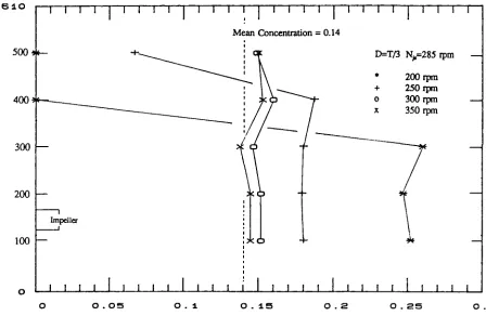
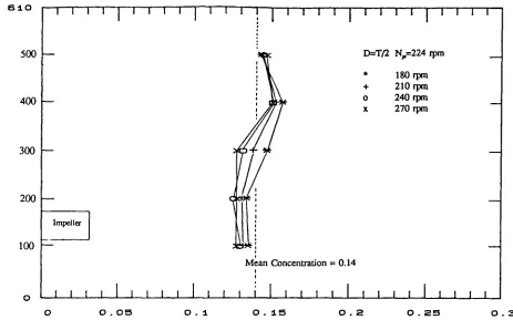
Experimental data are reported for solids suspension and distribution in four geometrically similar vessels with diameters equal to 0.31, 0.61, 1.83 and 2.67 m. Agitation was provided by a series of pitched blade turbines with impeller to vessel diameter ratios from 0.3 to 0.6 and pitched angles between 30° and 90°. The effect of impeller clearance on solids suspension was examined for a clearance range of T/4 to T/8. Dual impeller systems were also studied, covering two combinations (dual pitched and flat/pitched) and impeller spacing of half to two diameters apart. The majority of the experiments were carried out with 150-2 10 pm round-grained sand (density: 2630 kg m 3 and settling velocity: 0.015 m s') and tap water. Solids concentration was varied between 0.1 to 40% by weight.

Four parameters were measured; impeller speed, using an optical tachometer, power input, calculated from the shaft torque given by strain gauges, just suspension speed, ascertained both visually and by use of an ultrasonic Doppler flowmetering (UDF) technique and the local solids concentration, measured by a in-house solids concentration probe. In addition extensive flow visualisations were made with the 0.61 m vessel in order to establish both liquid and particles flow patterns during the experiments.

ACKNOWLEDGEMENTS

I am most grateful to my colleagues, Mr Robert Burnapp and Mr Kevin Lee, who proof read this thesis. They have been a constant source of help, support and inspiration during all these years in BHR Group Ltd, without them completion of this thesis would not have been possible.

Thanks are also due to:

My brothers and sister; Yan, King and Kin for sharing out my house duties and keeping my parents company while I was abroad.

My friends and colleagues; Lorna Brooker, I S Fan, Emily and Jack Ho, Steve and Marie-Ann Hobbs, Maha Soundra-Nayagam, Trevor Sparks, Mike Whitton and Ming Zhu for their encouragement and interest in this work.

Fred and Theresea Haines for providing me with a nice comfortable home.

My industrial supervisor, Andrew Green, for his moral support.

The author also wishes to thank the members of the Fluid Mixing Processes Consortium for their permission to publish part of the generic research results.

4

Human kind cannot bear much reality T. S. Eliot

Dedicated to my parents to whom I owe so much

that can never be repaid

All this I tested by wisdom and I said, "I am determined to be wise" - but this was beyond me. Whatever wisdom may be, it is far off and most profound - who can discover it? So I turned my mind to understand, to investigate and to search out wisdom and the scheme of things and to understand the stupidity of wickedness and the madness of folly.

6

LIST OF CONTENTS

Page No

Title Page

Abstract

2

Acknowledgements

3

Dedication

4

Nomenclature

10

Chapter 1 Introduction

15

1.1

Background

15

1.2

Research Needs for Solid-liquid Mixing

16

1.3

Aims, Approach and Thesis Layout

17

Chapter

2

Literature Survey

21

2.1

Solids Suspension

21

2.1.1 Zwietering's Empirical Correlation

21

2.1.2 Baldi et a! Turbulence Model

23

2.1.3 Mersmann et al Two Basic Laws of Solids Suspension

26

2.1.4 Shamlou and Zolfagharian's Average Velocity Model

28

2.1.5

Molerus and Latzel's Two Suspending Mechanisms

30

2.1.6 Wichterle's Characteristic Velocity Model

34

2.1.7 Other Models

36

2.1.8 Summary of the Suspension Models

39

2.2

Solids Disthbution

45

2.2.1 Relative Standard Deviation and Variance

45

2.2.2 The One Dimensional Dispersion Models

46

2.2.3 Buurman's Constant Froude No. Model

51

Chapter 3

Test Facilities and Methods

57

3.1

Base Configurations

58

3.2 The Vessels

58

3.3

The Vessel Bases

58

3.4

Baffles

59

3.5

Impellers and Clearances

59

3.6

Test Media

60

3.7

Impeller Rotational Speed

66

3.8

Shaft Torque

66

3.8.1 General Outline

66

3.8.2 Calibration and Accuracy

66

3.9

Minimum Speed for Solids Suspension

67

3.9.1 Visual Observation Method

68

3.9.2 Measurement of N with

an

Ultrasonic Doppler Flowmeter (UDF) 68

3.9.3 Calibration of the UDF Technique

70

3.10 Local Solids Distribution

71

3.10.1 The Solids Concentration Probe

72

3.10.2 Probe Calibration

73

3.10.3 Probe Location and Orientation

74

Chapter 4

Results and Discussion

83

4.1

Particle Flow Pattern

83

4.1.1 An Overall View

83

4.1.2 Flow Pattern at Vessel Base

85

4.2

Power Requirement for Solid-liquid Mixing

93

4.2.1 Solid-liquid Mixing Power

93

4.2.2 Just Suspension Power and Power Index

96

4.3

Effect of Impeller Diameter

106

4.3.1 Experimental Results

106

4.3.2 Just Suspension Speed

108

4.3.3 Just Suspension Power

112

8

4.3.5 Verification of Tip Speed Criterion

122

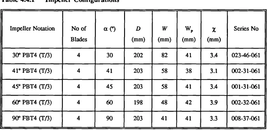
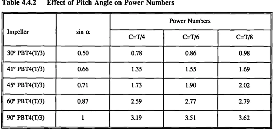
4.4

Effect of Impeller Pitch Angle

132

4.4.1 Power Numbers

132

4.4.2 Flow Pattern

134

4.4.3 Solids Suspension

134

4.4.4 Solids Distribution

140

4.5

Dual Impeller Systems

145

4.5.1 Power Consumption

146

4.5.2

Flow pattern

147

4.5.3

Solids Suspension

148

4.5.4

Solids Distribution

163

4.6

Scaling-up

173

4.6.1 Power Numbers

173

4.6.2 Solids Suspension

174

4.6.3 Solids Distribution

182

4.6.4 Comparison between the Two Scale-up Rules

183

4.7

Further Discussion

192

4.7.1 Overall Suspension Results

192

4.7.2 Comparing to the Suspension Models

193

(i)

Single Correlation Models

194

(ii)

Correlations with a Critical Dividing Parameter

197

(iii)

Models with a Continual Variation of Exponents

199

4.7.3 A Final Remark on Solids Suspension Modelling

200

4.7.4 Modelling of Solids Distribution

201

Chapter

5

Conclusions and Recommendations

207

5.1

Conclusions

207

5.2

Suggestions

for

Future Work

210

Appendkes

A

Solids Distribution Data for the Three Geometrically Similar Impellers

219

B

Solids Distribution Data for Pitched Angle Experiments

222

C

Solids Distribution Data for Dual Impeller Systems

224

D

Just Suspension Results Measured in Four Scales

232

E

Solids Distribution Results Measured in Three Scales

235

F

Just Suspension Results from Previous Study

245

Symbol A a A Am B C C CD Cii CL CM Ct Cv Cz D De,p d d F FB FD FL F g H h H,, NOMENCLATURE Meaning

A Calibration Constant A Parameter

A Constant

A Parameter Which Depends on Impeller Type Projected Area of the Particle

A Critical Constant for Just Suspension Condition Impeller Bottom Clearance

A Parameter Drag Coefficient

Local Solids Distribution at ith Speed and th Position Lift Coefficient

Mean Volume Fraction of Solids

Top Impeller Clearance in Dual Impeller Systems Volume Fraction of Solids

Mean Volume Fraction of Solids across Height z Impeller Diameter

Liquid Diffusion Coefficient Particle Dispersion Coefficient Particle Diameter

A Normalised Particle Diameter Thrust Force Generated by an Impeller Buoyancy Force Acting on the Particle Drag Force Acting on the Particle Lift Force Acting on the Particle Effect Weight of Particle

Gravitational Acceleration Height of Slurty

Height of Clear Liquid/Solid-liquid Interface Impeller Hub Height

Impeller Hub Outside Diameter

10 Units m2 m m m m2

s1

k A Constant

-K A Parameter

-L Length Scale of Large Energy Containing Eddies m

L0 Length Scale of Small Eddies m

L Characteristic Linear Dimension m

M Mass of Slurry kg

ML Mass of Liquid in Vessel kg

M Mass of Solids in Vessel kg

N Impeller Speed rev r' (or rpm)

n Number of Blades

-N Just Suspension Speed rev s (or rpm)

N,0 Just Suspension Speed by Visual Observation rev s' (or rpm)

Just Suspension Speed by Ultrasonic Doppler Flowmeter rev s 1 (or rpm)

np Number of Particles

-P Power W

P1 Power Index (P1 = Po s3 D24 ) m215

Pj Power Drawn by Impeller at N, W

Po Power Number ( Po = P /p N3 D5 )

-Poc Combined Power Number in Multiple Impeller Systems

-r Correlation Coefficient

-RSD Relative Standard Deviation of Solids Concentration

-S Geometrical Constant in Zwietering Correlation

-Si Modified Geometrical Constant

-T Vessel Diameter m

U Linear velocity m S_I

UI1 Axial Component of Local Velocity of Liquid at Point of

Incipient Particle Motion m

s4

Ufo Mean Upward Velocity Outside the Fictitious Tube m S'

Uf Eulerian Velocity of Fluid at z Direction m s'

Urn Mean Liquid Velocity near the Base of Vessel m

s1

Upz Eulerian Velocity of Particles at z Direction m

5'

Un Radial Component of Local Velocity of Liquid at Point of

Incipient Particle Motion m s'

UI Ut0, U11 Ut U.. V v, yr Vz w wp x z z

a

13 'YB Po LP$tat Cm ep C1 Cv lb icc Km K0 x p pay Terminal Velocity

Terminal Velocity at Stagnant and Turbulent Medium Shear Stress Velocity

Maximum Fluid Velocity Close to the Boundary Layer Volume of the Slurry

Fluctuating Velocity of the Critical Eddies Mean Radial Velocity

Mean

Axial

Velocity Blade Width

Projected Blade Width

Percentage Mass Ratio of Solids to Liquid in Suspension A Constant

Cartesian Coordinate in Axial Direction Blade Angle to Horizontal

A Constant A Constant

Characteristic Shear Rate at Vessel Base

Static Pressure Difference Inside Impeller Region Static Pressure Difference Outside Impeller Region Static Pressure Difference

Power per unit Mass

Power Dissipation for Entrainment of Single Particle Total Power Dissipation for Complete Suspension Average Power per unit Volume

Power per Unit Volume near the Vessel Base A Proportionality Constant

Characteristic Eddy Scale Corrected Conductivity Measured Conductivity

Conductivity of Water at Measured Temperature Conductivity of Water at Reference Temperature Blade Thickness

Density

Average Density of Vessel Contents

12 m s

m S'

m s m S'

m3 m S1

Ii

V

$ 'V

PL

Ps

kg m3 kg m3

Nm Nn12

kg m1 s1 m2 s' Density of Liquid

Density of Solids Standard Deviation Torque

Wall Shear Stress Dynamic Viscosity Kinematic Viscosity

Nondimensional Group for Pumping Characteristics Particle Resistance Coefficient for Free Fall at Stagnant and in Turbulent Medium

14

Dimensionless Groups

Ar Archimedes Number g ip d

v2 _PL

Eu Euler Number for Particulate Fluidisation d g (1 -C)2

3 P. U2

Fl Flow Number Q

ND3

Fr Froude Number N2 D

g

Fr Modified Froude Number N2 D 2 p L

d ip g

Ft Thrust Number F

p N 2 D4

Pe Peclet Number U H

D

Pe Modified Peclet Number U0 L

D,p

Po Power Number P

pN3D5

Re Reynolds Number P U d

It

Re1 Impeller Reynolds Number p N D2

Re Modified Reynolds Number N D3

vT

R; Reynolds Number for Shear Stress d U

CHAPTER 1: INTRODUCTION

1.1 BACKGROUND

Mixing is one of the most widely used unit operations in the chemical and allied industries. There is a general acceptance of the importance of mixing processes for the commercial success of industrial operations. In 1989 during a workshop conducted by the Mixing 3A of AIChE (Mixing 3A 1989), it was found that in many case studies presented, the monetary values of the solutions to the particular problems represented a saving in the region of $0.5 to $5M. Increasing process yields, avoiding the need for expensive and prolonged pilot plant development together with improved exploitation times in bringing new products onto the market, might represent a monetary value in the region of 1 to 3% of turnover for the chemical process industries, which for the USA was around $10 bn per year in 1989.

A stirred tank unit typically consists of a rotating impeller in a vessel. Fluid motion is promoted by the transfer of energy from the impeller into the process fluid. The process fluid may be single phase (eg viscous, Newtonian and non-Newtonian) or multiple phases (eg solids, liquid and gas) and, in some cases, physical changes may take place during the operation (eg suspension polymerisation and dissolution of solids in liquid).

Mixing processes are usually classified according to the type of the process materials, eg viscous liquid, solid-liquid, gas-liquid, liquid-liquid, etc, and of these, solid-liquid is certainly one of the most important. This has been highlighted in the survey conducted by the Mixing 3A Workshop which found that 80% of the chemical products made involved solid-liquid processing.

The main objectives of agitation in solid-liquid systems can be divided into three categories;

a) to avoid solids accumulation in a stirred tank

b) to maximise the contacting area between the solids and liquid

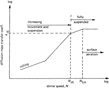
16 In many operations, it is essential to ensure that all the solids are kept in motion in order to prevent the building up of solids on the vessel base which may, in extreme cases, invoke system malfunction. Examples of such operations include settling tanks for filter cakes and absorber sump of a flue gas desulphurisation process. The stirred tank may also be used as a reactor, for example when catalysts are to be suspended for mass transfer operations. The mass transfer rate per unit energy input is at its maximum when the interfacial area between the solids and liquid is maximised. This happens when the fluid motion is vigorous enough to keep all particles in motion (i.e. at N, Fig 1.1.1). Even though the design objectives for (a) and (b) set out to achieve different goals, both require good knowledge of the just suspension speed (Np) prediction, that is the impeller speed at which no solid particle rests on the vessel base.

However operating the stirred vessel at the just suspension condition may not be sufficient in certain processes. For example, the ratio between the mean solids concentration in the vessel and that in the withdrawal tube depends on the position of the tube thus, solids distribution information is required to ensure good mass balance between inward and outward flow in a Continuous stirred tank reactor. Sometimes the product characteristics depend on the distribution quality, knowledge of which is then becomes vital for quality control.

In this work, flow pattern, power consumption, solids suspension and distribution for a wide range of geometries and scales were investigated.

1.2 RESEARCH NEEDS FOR SOLID-LIQUID MIXING

The Zwietering correlation

(1958)

is generally being accepted as the best correlation for just suspension prediction for low viscosity systems. This empirical correlation is based on more than a thousand experiments together with dimensionless analysis. However, there are a number of other correlations which are different and, in some ways, contradictory to Zwietering (eg effect of particle size and scale) and most of them have their own experimental data to back them up. Unfortunately, the discrepancies between many of these correlations are large.

models. Some of the assumptions adopted in establishing the theoretical models bear little resemblance to the actual suspension mechanisms. Therefore, more detailed observations of particle flow patterns would help to clarify this point. Scale-up data in literature is inadequate and extrapolation beyond the experimental range can be disastrous. For the just suspension conditions, published literature recommended oc 1" with n ranging from

0.5

(eg Kneule 1967) to -1 (eg Bourne 1974) (e = power per unit volume, T = tank diameter). For 100-fold change in scale, the two extremes give 1000-fold difference in power requirement prediction. An incorrectly sized mixing vessel could cause shut down of the whole plant and millions of pounds in lost production. Large scale data is urgently needed to verify the scale-up rules and the data should shed light on the validity of various models.

Another important feature for the evaluation of solid-liquid mixing performance is the distribution of solids throughout the vessel. However, quantitative information in this area is limited and mostly are confmed to low concentration in small vessels. The distribution of solids in an agitated vessel is a rather complex function of the velocity field, distribution of turbulence and solid-liquid interaction. Progress has been hampered by the difficulties in establishing a reliable measuring technique to be used in a wide range of geometrical set-ups which can provide useful information for modelling.

In the past agitation units were often greatly over-specified, in order to accommodate for the uncertainty in design. This may lower the yield (eg side reactions) and quality (eg particles breakage in crystallisation) of the desirable product. In additional, over-specification may lead to extra initial and operating costs Apart from that, treatment of undesirable products means extra production cost.

13 AIMS I APPROACH AND THESIS LAYOUT

18 To obtain an insight into the hydrodynamic conditions which govern the suspension and distribution of solid particles in mixing vessels.

To gain an understanding of the effects of some of the more important system parameters (eg geometric scale) on solid-liquid mixing.

To utilise the qualitative and quantitative information obtained, together with theoretical understanding to formulate and/or refme the existing models.

This work commences with a literature survey on solids suspension and distribution models (Chapter 2). Mathematical models developed in the literature to interpret the two phase flow mechanisms in stirred vessels are compared and contrasted. The survey highlights areas which demand more research effort and the type of measurements which ought to be made in order to verify/improve some of the existing models (eg particle flow pattern near the just suspension condition).

Chapter 3 describes the test facilities, methods and various physical and geometrical parameters that were encompassed in this programme. Three types of measurements were made in this work, namely just suspension speed (Ni), shaft torque for power calculation (t)

and local solids concentration at ith speed and th position (C1 ). Extensive flow visualisations were made during the experiments to aid interpretation of the results. The selection and verification of reliable and consistent methods for solids suspension and distribution measurements across a wide range of scale and geometries constitute a very important part of this thesis. The development and calibration of ultrasonic and conductivity techniques are also presented in Chapter 3.

contradict each other. One of the major tasks of this work is to validate the correlations by conducting a series experiments in four geometrically similar vessels (T = 0.31 to 2.67 m).

4-a)

0 () Cl)

_,

4- I-4-. (

E c

0

U) .4-

9--o

fully

suspended

surface aeration increasing

movement and suspension log

20

NJs NSA log

stirrer speed, N

CHAPTER 2: LITERATURE SURVEY

There are three objectives to this chapter. It generalises the present state of the art in understanding and designing a solid-liquid agitated vessel. It compares and contrasts the various mathematical models so developed to interpret the various phenomena taking place in the vessel. Furthermore, scaling up implications as well as particle-fluid mechanisms are commented upon in this section.

Solid-liquid mixing phenomenon in stirred vessels can be categorised into two regimes, namely solids suspension and distribution. Solids suspension is concerned with the last suspended particles on the vessel base and thus would be very geometry dependent, compared to solids distribution in which the bulk mixing of the vessel contents has to be taken into consideration. However, solids suspension and distribution are related, a solid particle has firstly be lifted by the fluid (suspension) before disthbuted into the bulk of the vessel contents (distribution).

2.1 SOLIDS SUSPENSION

2.1.1 Zwietering's Empirical Correlation (1958)

Zwietering published a classical paper on solids suspension in 1958 in which he adopted a rigid defmition for the determination of just suspension speed (Na). He defined thiS as being the minimum stirring speed at which no solid particle remains stationary on the vessel base for more than one to two seconds and claimed that this could be measured within an accuracy of 2 to 3%. This helped to bring many solid-liquid mixing research techniques together, as confusion had arisen in the past when researchers had not used a common N, defmition that would allow results to be compared.

22

9.3 x iO 3 Pa s were covered.

Zwietering proposed a list of 10 factors to determine the suspension of solid particles in stirred vessels

T vessel diameter

C distance between stirrer and vessel base D stirrer diameter

N stirrer speed d particle size

Ps density of solids PL density of liquid

V

kinematic viscosity

x

percentage mass ratio of solids to liquid in suspension g acceleration due to gravity

Following a dimensional analysis, a set of seven dimensionless groups were obtained:

TID,

TIC,

D/d geometrical ratios

N D2/v Reynolds number

N2 Dig Froude number

PSIPL density ratio

X solids concentration weight percentage ratio

The following relationship was obtained by analysis of the experimental data:

42

(ND2

1

PL N 2

D

I

ID

I

K (T

T

°.13

H Jgp

J J

...eqn(2.1.1)

The constant K and the exponent a depend on the type and position of the stirrer and the above equation can be rewritten as

45

N1, = s v°'

Ig

J

d 2 X°•13 D° 85 ...eqn(2.1.2)

The parameter "s" in eqn 2.1.2 is the geometrical constant and it is a function of the vessel and impeller configuration.

The Zwietering correlation is widely used for estimation of the just suspension speed. Its advantage is that it was based on a very large number of experiments and is dimensionless but, because it is an empirical correlation, it should not be applied outside its test range. Even though it has been re-confirmed by a number of researchers (eg Chapman 1981, Nienow 1968), the range of test parameters are still limited. So, it would be useful to expand the experimental conditions to discover under what circumstances this correlation would become invalid.

Zwietering used a mass ratio, X, defmed as the percentage mass of solids to liquid in the vessel, to quantify the solids concentration but one would expect volume fraction to be a better parameter to account for the fluid-particle effects.

2.1.2 Baldi et at Turbulence Model (1978)

Baldi et al (1978) postulated that the suspension of particles is mainly due to eddies of size similar to that of the particle diameter, and the energy transferred by these eddies to the particles is able to lift them to a height of the order of the particle diameter.

By performing an energy balance on the basis that kinetic energy imparted by the eddies is proportional to the potential energy gained by the particle, they showed:

PL V oc d ip g ...eqn(2.1.3)

where v' is the fluctuating velocity of the critical eddies

If the scale of the critical eddies is much higher than that of the eddies which dissipate their energy by viscous forces, and isotropic turbulence is assumed:

/ \113 F _CVb d I

...eqn(2.1.4)

volume, c

4

Po

_PL N

3

D5

e

=

_______

irT3

...eqn(2.1.5)

24

Schwartzberg and Treybal (1968) showed that the mean turbulent velocity in a stirred

vessel can be expressed by the above equation, even if the turbulence is anisotropic.

Baldi et at (1978) went on to assume that the local dissipated power per unit volume

near the tank bottom (evb) could be approximated to the average dissipated power per unit

Combining equations 2.1.3, 2.1.4 and

2.1.5

I

Td'

'

z

=

[PJ I ________

PL I.'. Po113 D

513

N J -

is)

From an analogy of the decay of turbulence behind a grid the authors deduced that:

z =

g

(

T

i

D

3

N.

Js),(

_()]

...eqn(2.1.6)

P.

_J

[PO"3 _{D513 N)} V

T

From experimental data at CID=1, eqn 2.1.6 becomes:

N.

oc i

0•17 (g Ap)° 42

d°

14

T

0.58

PL

Po°

28

D'89

...eqn(2.1.7)

Assuming Dfl and Po are constant:

N

oc

_°•'7

[LP

j42

X°

.

'

25 d

_A

₁

D -0.89

...eqn(2.1.8)

The semi-theoretical model (eqn 2.1.8) was verified by Conti and Baldi (1978) in a variety of flat bottomed tanks equipped with baffles; tank diameter varied between 0.122 and 0.229 m. The impellers used were 8-bladed disc and axial turbines. Seven classes of sand (42-540 .tm) and nine classes of ballotini (97-1200 tim) were tested. Both mono-modal and

bi-modal particle size distributions were employed.

The conclusion was drawn that the effect of particle size on N. is N, oc d,,', where the value of 'a' is between 0.14 and 0.16. However, they commented that particles with d < 200 im generally do not follow their model and suggested that the smaller particles are subject to a different suspension mechanism as yet not fully understood. Their results also suggested a strong clearance effect, and the exponents on eqn 2.1.8 will change with C/I). It is very likely that the solids suspension mechanism involves more than one hydrodynarnic regime and that these are a function of the geometrical configuration.

The authors justified their application of turbulent theory to solids suspension by arguing that the solid particles can be seen to be periodically picked up and re-deposited on the vessel base, a phenomenon difficult to explain using the alternative average velocity theory. Although this is a reasonable assumption, turbulence cannot be solely responsible for the suspension of solids. This has been demonstrated by filming of the suspension phenomenon in a viscous fluid (Shamlou 1991).

N2 D2 PL

Fr = ________ constant d p g

...eqn(2.1.9) 26 In the turbulence model, eddies are thought to be the primary means of getting the solids suspended and the intensity of turbulence within the reactor is a function of power dissipation per unit volume. Therefore, if turbulence is solely responsible for the lifting up of solid particles, one would expect a constant power per unit volume scale-up relationship as proposed in eqn 2.1.7 (i.e. Nfr oc D°67). However, after incorporating the experimental data into eqn 2.1.7, the authors proposed a scale-up relationship of N oc D° 9, which lies

between the constant power per unit volume and constant tip speed criterion. This casts doubt on their assumption that particles are solely picked up by turbulence.

2.1.3 Mersmann et at Two Basic Laws of Solids Suspension (1985)

Mersmann et al

(1985)

suggested that the mean specific power input (P) is dissipated into the vessel by two superimposed processes

:-(i) The consumption of power to counteract the sinking of the particles

in

order to avoid settling.

(ii) The generation of the discharge flow rate in the vessel so as to generate off-bottom suspension.

The 'to avoid settling' law is valid for small particles in a large vessel where the impeller has only to produce a mean upstream velocity greater than the settling velocity of the particles. By equating the two velocities, the stirrer speed which is necessary to avoid settling can be given as a constant modified Froude Number (Fr);

/

Hence N1, oc

f g

I d 5

D'

PL)

...eqn(2. 1.10)

N2D2p L

T

Fr

=

______

dApg d

...eqn(2.1.11)

27

solids distribution (eqn 2.2.26, Buurman 1985), even though the two authors were adopting

different approaches and trying to describe different mixing phenomena (Sec 2.2.3).

When suspending large particles, the authors suggested that the stirrer has to provide

sufficient kinetic energy in the liquid to compensate for the difference between potential

energy of the deposited solids and for homogeneous suspension.

I'

i.e.

N. F

g Ap

I

D°5

I'

PJ

.eqn(2. 1.12)

Eqn 2.1.12 suggests power input per unit volume has to be increased with scale in

order to maintain the solids in suspension.

To establish when the power input was being consumed to counteract the sinking of

the particle in order to avoid settling, as opposed to the circumstances when it was generating

discharge flow in the vessel to get off-bottom suspension, the authors used a characteristic

diameter ratio

(d,/T)

to distinguish between these two basic suspension mechanisms. The

ratio is a function of settling velocity, discharge coefficient, solids volume fraction, porosity

and the liquid depth to tank diameter ratio. If the real diameter ratio (d/F) is smaller than

its characteristic diameter ratio, it is relevant to assume avoidance of settling. On the other

hand, the off-bottom suspension law should apply if Cd/F)> (d/F).

This hypothesis was verified with a T/3 diameter marine-type propeller with a particle

diameter ratio 10 ^ (d/F)

^

10

(Mersmann 1985).

The transition point between the two

basic suspension laws was found to be at (d/F) - iO 3, which agreed well with Ditl's

transition region of

4.05 x

iO 3 ^ d/F ^ 1.7 x 102 (Diti 1985).

28

with T = 14 m with a d)T ratio of 7 x 10

6

_{. By plotting the ratio of Froude number as a}

function of the diameter ratio, they showed that a number of other researchers' results could

fit into their model very well (Fig 2.1.1). However, based on the plots in the paper, the

validity of this could not be substantiated.

2.1.4 Shamlou

and Zolfagharian's Average Velocity Model (1987)

Shamlou and Zolfagharian (1987) proposed a model for the estimation of the necessary

conditions for the incipient motion of particles, which was based upon the average velocity

of the fluid near the bottom of the tank and the hydrodynamic forces of lift, drag, buoyancy

and gravity acting upon the particles resting at the tank base.

They suggested that at the point of dislodgement, assuming that all the forces are

acting through the centre of mass of the particle, the moment of these forces about point 0

(Fig 2.1.3) must be zero, i.e.

xF - xFB = yF +

...eqn(2.1.13)

F,, = . CD p , U, A,,

and

FL = . CL P L U A,,

...eqn(2.1.14)

icd 3 PLUrnA

6

(pS-pL)g=

2

...eqn(2.

1.15)

i.e U

ocr' gLpd m

L PL (CL + CD)J

...eqn(2.1.16)

Shamlou (1990) refined the model by assuming that at the point of incipient

suspension of a particle, the rate of dissipation of fluid energy for particle lift-off is due to and

given by the total flow forces acting on the particle (Oroskar and Turian 1980).

= _{PL U U}

_O

_{, A}

_P

_(C

_L

_{+ CCD)} ...eqn(2.1.17)

He further assumed that the total rate of energy dissipation,

€,

required to entrain all the particles is proportional to the total number of particles, n,,, in the liquid. Since

U0,

oc Urn, A,, oc

d,,

2 and

(CL

+ CC

0

)

constant,

from 2.1.17:

Cl PL U

d,,

2

n

PL C,, 7'3

d

P

From the power number relationship:

P

=

_{Po PL}

N3 D5

Cvb

= k P = k Po PL

N3 D5

...eqn(2.1.18)

...eqn(2.1.19)

...eqn(2. 1.20)

Since

U0,

oc oc

Urn

and C,,b oc C,, combining eqn 2.1.16, 2.1.19 and 2.1.20:

Nfr A Po'0

Ig

J'

2

LPL

d, C,'° T

D 513 ...eqn(2.2.21)

This equation suggests a particle size effect of and a scale-up effect of D on N (assuming D oc _{7), as compared to d° 2 and D as proposed by the Zwietering} correlation. The author confirmed his model by testing several 4-bladed pitched blade turbines in a 0.24 m diameter glass vessel. The particle diameters ranged between 175 and

3015

Jim. Their results produced a value of N proportional to d°' 7 D° 67 which is in good agreement with the theoretical model.

30 Now the question is, could the solid particles be lifted up by turbulence or even a combination of both flow and turbulence? If so, should the exponent on D be different? It is interesting to note that the exponents on Shamlou and Zolfagharian's model are very similar to that of Baldi's, even though their initial assumptions differ. The exponent of -0.67 on D (constant power per unit volume) suggests that for whichever type of suspension mechanism is involved, its intensity is a function of power input.

2.1.5 Molerus and Latzel's Two Suspending Mechanisms (1987)

Molerus and Latzel (1987) suggested that the suspension of solid particles in a stirred vessel is governed by two different mechanisms, depending on the Archimedes number. The fust one defmes the complete suspension of fme grained particles (Ar ^ 40) being attained at sufficiently high shear stresses in the wall boundary layer of the vessel. The second criterion, generally applicable to coarse grained particles (Ar> 40), is based on an analysis of the pump characteristics of an agitated vessel.

(i) Fine Particles (Ar ^ 40)

The authors observed that the settling velocity of 66 pm glass ballotini suspended in water was almost two orders of magnitude lower than its circulation velocity in a 1.5 m diameter vessel. This leads to the conclusion that the region responsible for the complete suspension of the particle is the wall boundary layer of the vessel where the local fluid velocities are similar to the particle settling velocity.

They took the maximum fluid velocity U,. close to the boundary layer as a reference velocity. Measurements in three geometrically similar vessels (T = 0.19, 0.45 and 1.5 m) showed a linear dependence of U_ on the circumferential stirrer velocity (ie U_ oc N D).

I 3

It

U _¶ =i

(PL

...eqn(2. 1.22) This gives the shear stress velocity of:

From the wall shear stress relationship described by Schlichting (1965)

= 0.182 v°' U..° 9

r°•'

...eqn(2.

1.23)

In order to establish the flow forces exerted on particles settled in the boundary layer, the shear stress for a particle layer is assumed to cover the wall surface and hence;

7td2 itd3

( 4 ) t=i p( 6)g ...eqn(2. 1.24)

and _Re =

[dutJ

Combining eqn 2.1.22, 2.1.24 and 2.1.25

-

___

Ar Re—

JJ-

3

...eqn(2.1.25)

...eqn(2.1.26)

The above equation was confirmed with tests on various sizes of glass and steel beads (34 ^ d ^ 1937 j.tm), with a concentration range of 0.5 to 30% by volume, in geometrically similar vessels (T = 0.19, 0.45 and 1.5 m). Tap water and water/ethylene glycol mixtures

were used as the test fluid. The experimental results agreed with the model in the regime Ar ^ 40.

From equation 2.1.26;

I'

I _d g Ap I

U oc " _{...eqn(2.1.27)}

32

Substituting into equation 2.1.23;

g Ap

v-°

•

"

T°" -

P,. )

Since U..

ocND,

thus;

_

g _p

I

N [d ___ 36

PL

J v°" D' T°1'

...eqn(2.1.28)

...eqn(2.1.29)

The above equation suggests a particle size effect of

N, oc d°

6

and a scale effect of

N oc D°29

for geometrically similar vessels, but that just suspension speed is independent of

solids concentration.

(ii)

Coarse Particles (Ar> 40)

Molerus and Latzel (1987) also developed a criterion for predicting minimum speed

for solids suspension for coarse particles, which was based on:

(i)

An appropriate representation of the dependence of the drag on fluidised particles on

the concentration and

(ii)

An analysis of the pump characteristics of an agitated vessel, analogous to the

theory of similarity of fluid-kinetic machines.

They started by assuming a fictitious tube of a diameter D around the impeller.

Assuming complete fluidisation outside the impeller region, the static pressure difference

required by the stirrer, iP can be given by:

&'J at =

AP0 -

...eqn(2.1.30)

=

1

Cp5-s-(l-C)pL]gH-pgH

UJo

(1-C,,) D N ...eqn(2. 1.35)

(1-C,,)2 AP =

[(I-C,,) PL C,, Ps U102

...eqn(2. 1.36) Where P1 and P0 are the static pressure difference between the top and bottom, inside and outside the impeller region respectively.

From the Euler Number for particulate fluidisation

Eu = ± .e. ..! (1-C,,)2

3 P. U2 ...eqn(2.1.32)

Eu = ±_Al' _fi d (1-C,,)2

3PLL'JOH cv

and for constant Eu, from eqn 2.1.32:

p

d

g

UIO2 oc

(1-C,,)2

PL

...eqn(2. 1.33)

..eqn(2.1.34)

By comparing the flow in an agitated vessel with a pumping system, the authors generated two nondimensional groups to describe the pumping characteristics of two-phase flows in agitated vessels

34 It was found that (,)2.77 for Ar> 40, hence:

(1-C,)2 AD ( 10

2.77

LU

__________________ oc ________ [(l-C,)p + , _P]

u

2 _{L(1_c,)} D N}

...eqn(2.1.37)

Jo

Substituting and Uf0 and for a given scale, (1-C,,) _1k + C, _Ps

constant

N. Ap d IC, H P L

.36

P

i

E

)2

)

d

i.e. _{Nfr (g ip)°3}

[J.14

(C, jj)036 D-' ...eqn(2.1.38)

The above equation suggested the influence of particle size and scale on N,, were and DOM. It is interesting to note that their effect of liquid density on N, (i.e. N,, oc _PL°'4)

is much smaller than that are proposed by the other researchers. Moreover, the dividing criterion of Molerus's model (Archimedes Number) depends on densities, particle size and viscosity but not tank diameter as proposed by Mersmann nor power input as in Diii's model. Influence of solids concentration is included in Molerus's model only when Ar> 40, for Ar ^ 40, the authors observed no dependence of N,, on solids concentration.

2.1.6 Wichterle's Characteristic Velocity Model (1988)

Wichterle (1988) developed a theoretical model for solids suspension based on the comparison of the terminal settling velocity of a particle and the characteristic velocity of the agitated liquid around the particle at the vessel base. He suggested that the flow acting on a particle of diameter d. lying on the bottom can be characterized by a velocity B (Fig 2.1.4) and V8 = 'YB d. If VB is higher than the settling velocity of the particle (U,), the particle will

be suspended and thus, the suspension condition can be related by a critical value B,, which is a function of particle shape;

B. = 'y 8 d ...eqn(2.l.39)

d

N = _______

18 + 0.6

...eqn(2.1.45)

The relationship between the particle diameter and settling velocity was related by a

semi-empirical correlation:

U, dP pL Ar

(18

+

0.6

Ar°5)

He defmed a normalised particle diameter, d'

Ar = = d PL

g

...eqn(2.l.40)

...eqn(2.1.41)

From a laminar boundary layer of an impinging jet

lB = N A Re1°5

.eqn(2. 1.42)

Where A,, is a minimum value of a constant A, which is dependent on the

geometrical configuration of the mixing vessel according to the author's electrodiffusion

experiments. A,, is equal to

2.5

for disc turbines at T/3 clearance and 3.5 for 6-bladed

pitched bladed turbines at T/2.5 to T/5 clearance.

Wichterle then introduced a dimensionless critical impeller speed for just suspension,

N, where:

(PL

Ni;=Nv- 1 gp

J

D2T

.eqn(2. 1.43)

From equations 2.1.40, 2.1.42 and 2.1.43

•

(Br

36 The proposed correlation was verified by plotting other researchers' results in the format of N, against d (Fig 2.1.2). From open publications (Einenkel 1980, Paviushenko 1967, Rieger 1982, Staudinger, Tay 1984 and Zwietering 1958), a value of 10 ± 2 was estimated for B,.

The author's model predicts that in the whole range of variables, a single-power function N oc D 213 (D/T) 3 applies (eqn 2.1.43), which suggests a constant power per unit volume scale up rule. However, influences of other parameters (d 1.1, _{PL and p) on N are} a function of the normalised d, i.e. Ar' 3 (eqn 2.1.41). A single power law relationship will be given for a constant Ar. Work conducted by other researchers had already suggested that the effect of particle size on just suspension speed is not a simple single power law relationship, but divided by critical values, which could be a function of Ar (Molerus 1987, Rieger 1982). Wichterle further proposed that there were not just two different exponents on d, but a continual variation of exponents both on d and other parameters.

The scale-up rule of D on just suspension speed is somewhat questionable. The reasons are two fold; firstly, the author did not deduce the scale-up relationship theoretically but instead, assumed a dimensionless critical speed (eqn 2.1.43) for solids suspension without proof. Secondly, the other researchers' data with which the author tested his model were all obtained from a rather limited range of vessel sizes. If the particle is being picked up by flow rather than turbulence as the author suggested, one would expect scale-up to be more likely to be governed by constant tip speed criterion.

2.1.7 Other Models

N = 1.782 X22 _{(T)2 __1__ [} D 2T-D

2d (2 g ip) [...L +

3p _L

HX 100 (p^X _PL)

...eqn(2.1.46) Although the above equation showed very good agreement with the experimental results, its fundamental assumptions were somewhat questionable and its range of application should thus be restricted to that within which the empirical constants were established. However, the approach adopted by the author does look somewhat more appropriate to describe the distribution of solids in a stirred vessel.

Subbarao and Taneja (1979) proposed a simplistic model based on a balance of the fluid velocity and particle settling velocity for a propeller agitated system. The particle settling velocity was estimated from a correlation for the porosity of a liquid fluidised bed as a function of liquid velocity. Their model indicated a negative exponent on d in all circumstances which is questionable.

Kolar (1961) proposed that the mixing energy at the critical condition can be related to the potential energy of the particles (i.e. power input equal to the effective weight of solids times the particle free falling velocity) and that the particle settling velocity is proportional to the impeller tip speed. The author tried to account for the effect of turbulent dissipation on the settling velocity by the relation;

•, U 2 = UO2 ...eqn(2. 1.47)

However, his assumption is too simplistic to describe the actual suspension phenomenon.

...eqn(2.1.48)

38 They postulated that the dividing criterion between different mechanisms can be defined by the relative

size

of particles to characteristic eddies. For the smaller particles the characteristic scale

can

be given as:

Thus

"4 Po 1dp '"1\'_D2

PL 1

(r

3i

nHJ

J

4

...eqn(2.1.49)

Results from thirty eight set of experiments were correlated, to evaluate

the

critical particle diameter. Based on statistical

analysis:

0.45

(d ' (T

-0.56

Re cc Ar

(

TJ

J

...eqn(2. 1.50)

For large particles;

(d / Th) ^ 32, 13

=

-1.42

=

Ni,, cc d°°7 and D°58

For small particles;

(d, / r) <32,

1

3

=

-1.25

=

N cc d°'

and

D°75

p N D413

_________ = constant g p

d"

...eqn(2.1.52) Musil and Vik (1978) based their theory on the balance of the liquid and particle kinetic energies, which was very similar to Kolar's initial assumption. Their results were expressed in the form of a critical Reynolds Number, which is a function of Archimedes and Particle Reynolds Number. However, their mathematical reasoning for the derivation is impossible to follow. It has been pointed out that there are a number of mistakes in Musil's physical assumptions and mathematical treatment (Diti 1980).

Buurman et a! (1985) employed a similar hypothesis to that of Baldi et al, relating the kinetic energy of the eddies to the potential energy of the particles;

p v 2 d oc g ip d ...eqn(2.1.51)

The equation led to the form of a modified Froude Number, which suggests a constant power per unit volume scale-up relationship;

2.1.8 Summary of the Suspension Models

According to the suspension mechanisms, the theoretical models which have been reviewed so far can generally be classified into two categories; namely those in which particles are believed to be picked up by turbulent eddies (eg Baldi 1978, Diii 1985) and those in which particles are believed to be picked up by fluid flow (eg Shamlou 1987, Wichterle

1988). There is a third category in which the suspension model is not based on an independent mechanism but is simulated by another phenomenon of which the researchers had more modelling experience, such as pump flow or fluidisation (Molerus 1987). This section will compare and contrast models derived from the first two categories, as they gave a better fundamental understanding of the suspension mechanism as compared to the simulation models.

40 average velocity concept. However, the turbulence models on their own cannot explain why axial flow impellers, which have a lower power number than their radial flow counterparts and hence, a lower level of turbulence, are nevertheless able to suspend solids at a lower energy input, bearing in mind that an axial flow impeller is generally flow dominated. Moreover, Al-Dhahir (1990) has shown that solids suspension is possible with viscous liquid operating in the laminar regimes well before turbulence sets in.

Although both of these theories display considerable merit, there remain a few questions to be answered. In the turbulent model, mean energy dissipation is assumed and the related kinematic quantities are usually derived according to the concepts of Kolomogoroff's theory of homogeneous turbulence. However, it is obvious that the energy input does not dissipate uniformly throughout the vessel and there is as yet insufficient knowledge of the dissipation intensity in the vicinity of the bottom where the solid particles are to be suspended. Moreover, the damping effect due to the presence of solids is extremely difficult to quantify. It has also been reported (Squires 1990) that the turbulence field was modified differently by light particles than by heavy particles. Moreover, the validity of Kolomogoroff's theory in a mechanically agitated vessel has yet to be verified.

On the other hand, the velocity model approach also presents problems. The flow model assumes that regardless of the flow condition in the core (turbulent or laminar), flow near the base is not turbulent during suspension. Most of the models that have been reviewed were too simplistic to quantify the complex interaction between fluid flow and geometry. For example, flow within the core of the vessel could be very different from flow near the vessel base. The location of the last suspension region depends on a combined effect between vessel base and impeller discharge flow. The influence of geometrical configuration on

N,

may vary from one location to another due to differences in flow nature. If one wishes to explain the periodically picked up and re-deposited motion of the particles on the vessel base by means of the velocity model approach, one has to accept that the fluid velocity must be unsteady, varying considerably across the vessel base. Therefore, a more accurate way of relating the impeller rotational speed to the fluid flow adjacent to the solid particle to be suspended is necessary.

reasonably well. They suggest v and p exponents ranging from 0.11 to 0.17 and 0.42 to 0.56 respectively. However, almost all the turbulence models suggest an exponent of 0.17 (eg

Baldi 1978) and -0.67 (eg Buurman 1985) for the particle size and scale-up effect and the flow model recommended an exponent of 0.5 (eg Mersmann 1985) and -1 (eg Molerus 1987) for the corresponding effect. Incidently, most of the exponents reported in open literature lie between 0.14 and 0.5 for particle size effect and -0.67 and -1 for scale-up effect. This makes one wonder if the solid particles are being picked up by a combination of these two effects and that the magnitude of the exponent is dependent upon the proportion of particles being picked up by each of the two mechanisms.

Most of the models formulated have not allowed for the effect of liquid viscosity and solids concentration. These are extremely important, for both the liquid velocity and turbulence intensity will be modified by these parameters. Shamlou (1990) considers the concentration effect by relating the number of particles in the vessel to the power input and he found that N, C,,''3. Buurman (1990) suggests that the effect of solids concentration is a function of liquid and solid density, particle size and scale of equipment. Until models have been developed which account for all these complex interactions, it is unlikely that any pure theoretical model will be able to bring all the available experimental data together.

I

hi

-

bO E _E

c 'S

-.' U

S ' )

g.

o 0

? °

o - C) C)

z' U

'S

r- C\ N

r-00 O 00 - '1 O 00 O O

qqq '9q q qq

cn

- • I I I I

o

-N N

a. - - _{' C)}

I,) ir

.9

< C C 0 _d C

___ ___ ___

-N

-- I - I I

-d

-C)

a)

.

9

.

.2

.° _{. -} C) .

•a2:

00 In

In 00 N N

00 00 00

- N

-- (I)

._ =

. U

C) .

._... 1,0 —__—,

1

'- -,

• •

- L

0,1

Subscripts s: with solids w: in water

Fig 2.1.1

I

e4

1

0.1

avoidance of settling

m=0

Fr = constant •%

Niesm Eanenkel

Con 1978 Rieger 1982

Kneule 1967

0, i;o

d

_IT

10

T

Ratio of Froude Numbers as'a Function of Diameter Ratio according to Void & Mersmann's Model (1986)

10

EINENKEL 8O ZWIETERING 1958

1978

- - jER 1977

TN l9Zh

—

SUGGESTED-7 - N*

MODc/'

-—

-, I

0.1 •1 10 100 1000

d E d (Qg/J2)hh'3

ig 2.1.3

Force Balance for

amlou's Average Velocity Model

;=yix

Un

Settling

Suspending

44

1-.

4FW

Terminal Settling Velocity,

U1

/

_4.

Characteristic Velocity at the Bottom

2.2 SOLIDS DISTRIBUTION

The distribution of solid particles in a stirred vessel can be described by means of the degree of homogeneity within the vessel contents. Very often, a uniform dispersion of solids throughout the mixing vessel is necessary to ensure adequate exposure to the process conditions. However, the amount of research in this area is limited when compared to the study of solids suspension, attributable mainly to the difficulties in the development of a reliable experimental technique (Sec 3.10). This part of the survey will focus on major experimental and theoretical fmdings in solids distribution literature.

2.2.1 Relative Standard Derivation and Variance

Relative standard derivation (RSD) is very often quoted to quantify the distribution quality of solids in multiphase stirred vessels. It is a measure of the deviation of the local solids concentration from the mean holding solids concentration. The magnitude of RSD decreases as the distribution becomes more homogeneous and perfect homogeneity will give a zero value.

Defmition of RSD in open literature can differ slightly, depending on which statistical mean is taken (number of samples equal to n for sample mean and (n-i) for population mean). Throughout this study, the following defmition is adopted:

RSD- 1 ( 1- (n-i)

(C - CM )2

J

...eqn(2.2.l)

C1 is the local solids concentration at th position and th speed CM is the mean bulk solids concentration from calculation

n is the number of sampling positions and n is equal to 5 in this investigation

In some literature, variance (a) is used to define the distribution quality and the relationship between variance and relative standard deviation is

46

2.2.2 The One Dimensional Dispersion Models

In modelling the distribution phenomenon, most researchers based their analysis on a one-dimensional sedimentation-dispersion model. This can be derived from a general diffusion equation (Appendix G). To model the distribution processes, both the solid and liquid phases are taken as an upward moving continuum and a particle diffusion (dispersion) coefficient is employed to account for the relative movement between the two phases. This coefficient is a function of power input, physical properties and geometrical configurations.

Barresi and Baldi (1987) used the monodimensional model and assumed the solids phase to be a continuum. Neglecting the inertia forces, the local mean-time solids velocity in the axial direction is a vectorial sum of the liquid velocity and the terminal velocity:

U,,, = - U ...eqn(2.2.2)

Since the net flow rate of the liquid through a section is zero, an integration of equation 2.2.2 over a generic section leads to:

Upz = Uts ...eqn(2.2.3)

From the general diffusion equation, assuming U oc U:

dC U 0 C +D

'' dz

...eqn(2.2.4)

Therefore, the local concentration depends on They introduced a modified Peclet Number (Pe) to describe the local concentration. With L being a characteristic linear dimension of the system, Pe is defined as:

UL

Pe = ______ ...eqn(2.2.5)

U₁₀ Peoc

Po"3ND

...eqn(2.2.6)

47

By relating the power input to the turbulent scale:

They went on to define a K parameter, which is the inverse of the modified Peclet

Number, i.e.

K

=

Po"3 N D / U,. This is

so defmed in order to stress the fact that the

dispersing phenomenon is not due solely to the turbulent diffusion, but also to the anisotropic

turbulent motion. By plotting relative standard derivation against K/X°'

3

to account for the

concentration effect, they showed that the suspension quality can be correlated as a function

of the stirrer speed (Fig 2.2.1). This is implying a constant tip speed scale up relationship for

equal quality of solids distribution. It is important to point out that their plots of RSD versus

K/X°'

3

for different impeller types can be somewhat misleading. Firstly, their impellers were

confined to T/3 diameter only and therefore, their proposed effect of D on RSD is yet to be

validated. Moreover, by overlaying their plots it can be shown that their

results did not confirm RSD oc Po 3

(Fig 4.4.8).

Magelli et a! (1987, 1989, 1990 and 1991) adopted the simplified diffusion equation;

d2C dC

-D __Z+UZO_{ep dz}

2 ' dz

With the boundary conditions:

dC

UC -D - =0

(z'.0) _dz

(gO•)

...eqn(2.2.7)

.eqn(2.2.8)

0

CM !

5

Cz) dz

...eqn(2.2.9)

H

The solution of the equation is:

C j = Pe —Pe z

_{.eqn(2.2. 10)}

RSD = (C -CM n

...eqn(2.2.

11)

48

The authors suggested that suspension inhomogeneity can be characterized by the

relative standard deviation (RSD) of the solids concentration with respect to the mean value

and RSD can be expressed as a function of Peclet number (Pe). Note that their defmition of

RSD differs slightly from that presented in this investigation.

RSD=1 e'-1

_iJ°

2

(e r'- 1)2

...eqn(2.2.12)

and

Pe= -UH

...eqn(2.2.13)

D '4'

They conducted a series of experiments in a 0.23 6 m diameter stirred vessel, with

various liquid depth (2.3 ^ HTF ^ 4) and impeller combinations. A variety of solids and fluids

were also tested. They established that a single interpolating line can be obtained for all the

geometries studied, for each particle

size and

liquid viscosity. Therefore, they proposed the

following relationship in order to account for the physical and geometrical parameters;

Pe

=

A.

___

I____

NDJ

...eqn(2.2.14)

Based on test results from Rushton turbines, the exponents on (I-hF) ratio and

(v

3

/cm

d) were found to equal 2 and

0.095

respectively. They observed a lower distribution

efficiency of radial impellers in comparison to axial impellers. Incorporating results from

axial impellers (with the above two exponents kept constant), further analysis yielded the

following correlation (Fig 2.2.4):

..'i17

H (0

_I

(v3

Pe =

330

T

J

D ) d:J

or depletion of the particles;

dC

UC +D =0

'' dh .eqn(2.2. 17)

d (lnC) - - U,1

dh D_e,p

...eqn(2.2.18) By assuming a power law dependence of RSD on Pe, equation 2.2.12 can be simplified as:

RSD = 0.29 Pe°'92 for 0 Pe ^ 6 _{...eqn(2.2.16)}

An important contribution of Magelli et al's work is the successful demonstration that all physical and geometrical parameters they have tested so far can be presented in terms of a single adjustable parameter (Pe - Peclet No, eqn 2.2.14). The relative standard derivation of solids concentration can be related to the Peclet number by a power law approximation. Thus, the homogeneity of a solids distribution system can be predicted from equation eqns 2.2.15 and 2.2.16. Since , oc _{N3 and therefore Pe cc N446 and RSD cc N'24. A scale up}

implication of N cc D° 93 can be deduced from these two equations.

Shamlou and Koutsakos (1989, 1991) conducted a mass balance on the particles over a thin horizontal section of the liquid in the vessel, and assuming that there is no accumulation

Where D4, and U are the dispersion coefficient and settling velocity of the particles in suspension. Eqn 2.2.17 can be rearranged into the format;

Thus, a plot of (in C) against height, h, is expected to be a straight line with a slope of -U, / To simplify eqn 2.2.17 further, the authors proposed the following assumptions;

- The particles in suspension were small and thus behaved in the same manner as the agitated liquid. So the particle diffusion coefficient, D o.,,, may be expected to coincide closely with the liquid diffusion coefficient,

i.e. De4, cc _{...eqn(2.2.19)}

8IBL LONDON

50

-

Homogeneous and isotropic turbulence exists in the core of the agitated vessel.

i.e.

N3D5

...eqn(2.2.20)

£

T2H

- Away from the discharge zone of the impeller, the mean rate of energy dissipation

in the core of the vessel is directly proportional to the total energy input per unit mass.

- The relationship for small eddies of scale

_L

in the Kolmogoroff range applies to the

larger energy containing eddies of scale L.

i.e.

v'

(

Cm L

0 )"3oc

(CmLe)"3

..eqn(2.2.21)

Assuming

U

ec

U,47 ,

and for a fixed tank/impeller geometry:

U,: Uu,

_{...eqn(2.2.22)}

By introducing the ratio d/D, the above equation can be expressed in dimensionless

form by using a Peclet number defined as U d.JD

U,: d _(J,,

_{...eqn(2.2.23)}

D ND

The authors therefore concluded that the distribution of particles in the agitated liquid

can be characterized by a single parameter, namely the ratio of the turbulent diffusion

coefficient of the particles to their terminal settling velocity (Fig 2.2.2). All other properties

of the system, such as particle size and density, impeller diameter and speed and fluid

properties exert their effects only through the value of this ratio. According to eqn 2.2.23, if

the distribution quality is to be maintained, the tip speed of the impeller across scales has to

be a constant.

All three models used the settling velocity (single particle in still fluid) to account for the solids and liquid properties. Baldi et a! (1987) used RSD oc to account for the effect of solids concentration in homogeneity, an arbitrary correction taken from Zwietering's correlation for solids suspension which seemed to work well for low solids concentration. Apart from that, no analysis has been conducted to include this important parameter in their models. The models all point roughly to a constant tip speed scale-up implication. This was deduced by testing impellers of different diameter in the same vessel (ie varying DIF ratio). If turbulent eddies were responsible for the distribution of the solids as was assumed, one would expect power per unit volume must be kept constant between scales in order to produce the same degree of turbulence. Moreover, Buurman (Sec 2.2.3) correlated the solids distribution data taken from various sized vessels (0.24 5 T S 4.26 m) and he concluded a

N oc _{D° 78 scale-up relationship. It may be the case that constant tip speed criteria work for}

different D/T ratios but not necessarily so if the different tank sizes were used with DTl' maintained constant. This is a subject of further investigation in this thesis.

2.2.3 Buurman's Modified Froude No. Model (1985)

In order to achieve a certain degree of homogeneity in a stirred vessel, the solid particles have to be lifted up from the vessel base and then transported throughout the whole vessel. Buurman et a! suggested that it is not only the eddies of the inertia! sub-range that are isponsible for the mechanism but that the largest eddies (i.e. circulation) also play a role.

They assume the fluctuating velocity, which is responsible for entrainment of the particles, to be proportional to the circulation velocity, i.e to the impeller tip speed.

V oc ND ...eqn(2.2.24)

From an energy balance between the kinetic energy of eddies and the potential energy of the particles: