Combined full field stress and strain measurement methods
for granular materials
J. Dijkstra1,aand W. Broere1
Delft University of Technology, Geo-Engineering Section, P.O. Box 5048, 2600 GA Delft, The Nether-lands
Abstract. The current paper re-introduces the photoelastic measurement method in ex-perimental geomechanics. A full-field phase stepping polariscope suitable for geomechan-ical model tests has been developed. Additional constraints on the measurement and me-chanical setup arising from geomeme-chanical test conditions are outlined as well as the op-portunity to measure the displacement fields in the sample with digital image correlation. The capability of the current setup in retrieving the stress and strain field in a granular material is demonstrated.
1 Introduction
Performing full field stress measurements in natural soils is very difficult. For a decent spatial res-olution the size and amount of the required sensors embedded in the soil simply would negatively influence the characterisation of the stress state. The physical size of the sensors prohibits a realistic failure mechanism. Full field soil stress measurements, therefore, can only practically be obtained with a photoelastic measurement method.
Photoelasticity is a well established measurement method in experimental mechanics for obtain-ing the stress field in photoelastic materials (i.e. a transparent material with a noncrystalline molecular structure). The method, introduced in engineering in the beginning of last century, e.g. [1], was pio-neered in geomechanics by [2] [3], [4] . Over the years the originally qualitative methods gradually became more quantitative by the introduction of more advanced measurement equipment and post processing which is summarized in [5].
Interestingly, these newer methods stayed in the realm of experimental mechanics and did not enter geomechanics. Some ideas were addressed in the work of [6] and [7] and more recently in physics by [8] and [9]. However, stress measurements in granular media using photoelasticity are still very limited.
The current paper aims to re-introduce a more advanced quantitative phase stepping measurement method into geomechanics and combines it a with the digital image correlation method to measure the displacements fields (using the natural contrast of the granular material), e.g. [10]. Together these methods could potentially offer the combined stress-strain response of the granular material.
2 Photoelastic Measurements
The stress measurements consists of three steps: (1) acquiring the photoelastic parameters in the sam-ple by measuring the retardation and the isoclinic angle of the polarized light, (2) unwrapping the phase of this experimental data, (3) deriving the individual stress components in the stress seperation routine.
a e-mail:[email protected]
© Owned by the authors, published by EDP Sciences, 2010 DOI:10.1051/epjconf/20100622020
Before presenting the details of these steps in more detail, first the limitations of the geotechnical setup will be discussed.
2.1 Limitations imposed by geomechanics
Compared to homogeneous materials generally used in experimental mechanics, the granular mate-rial as studied in geomechanics poses additional challenges. The particulate nature results in a non-homogeneous sample with voids between the grains. These grains are not bonded and therefore will require a plane strain strongbox to contain the sample. The front and back wall of this strongbox should be transparent and have minimal influence on the photelastic effect. The stress-optic law is equally applicable in plane-strain conditions as shown in [11].
In the current study the granular material, or soil, is replaced by grains of a photoelastic material. A strongbox is filled with crushed glass particles. The voids are filled with a liquid, Exxon-Mobil Marcol 82, which is matching the refractive index of the glass, in order to prevent light scatter in the sample. The other properties of this matching liquid, such as viscosity and density, are as close as possible to water. In [11] the similarity in mechanical behaviour between broken glass and sand is shown using triaxial test results. The crushed glass grains, however, are more angular than sand and as a result the aggregate properties are slightly different (as are strength and stiffness of the individual grains, which could render the material more prone to crushing). On the whole, they are a reasonable substitute material to investigate sand behaviour.
A remaining fundamental consideration is that multiple grains are stacked over the thickness of the sample. For the current setup, where the light passes multiple grains, this implies that the observed light intensity is the sum of the light intensity changes (due to the mechanical shear stress) in every single grain along the path of the light ray. The stress field, therefore, is a 2D stress representation in the plane perpendicular to the light ray of an averaged intensity reading over the depth of the sample. This 2D cross-section does not present the full stress tensor. Out of plane stress components are not detected, i.e. the stress state is measured in a plane perpendicular to the light ray as the method is insensitive for polarization changes along the light ray.
The photoelastic effect is measured using a transmission polariscope. This apparatus projects light with a pre-defined polarization state on the sample. The stressed sample will alter the polarization of the incident light and this alteration of the light polarization is subsequently measured. For seven orientations of the wave plates and the polarizer in the polariscope a light intensity measurement is required in order to collect sufficient data for the subsequent analysis.
The size of the physical models as used in geomechanics tends to be quite large in order to preserve a reasonable grain size to structure size ratio. This size typically is larger than the size of available retardation and or polarization plates. Therefore, most of the methods listed by [5] are not suitable without modifications. The most straightforward modification, moving the sample or the polariscope with respect to each other, are not feasible options due to mechanical limitations and would in any case significantly increase the required number of polarisation state acquisitions. The new setup described here does not need to move sample and polariscope with respect to each other and only needs seven acquisitions for the full field. This reduces the acquisition time considerably and improves the spatial resolution.
2.2 Acquiring the photoelastic parameters
The polariscope used in this research consists of two linear polarizers and two retardation plates (also called λ4 plate) and is shown in Fig. 1. The proposed optical arrangement and configuration of [12] is used for the measurement of the photoelastic parameters in the sample, i.e. the retardationδand isoclinic angleφin Fig. 1. This method allows to compensate for poor wave plate performance.
camera
sa
m
p
le
p
ol
ar
iz
er
re
ta
rd
er
re
ta
rd
er
p
ol
ar
iz
er
light source
R
γ(∆)
P
π2
R
β(∆)
R
φ(
δ
)
P
θFig. 1. Arrangement of optical elements in a polariscope.
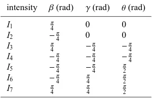
Table 1. Seven configurations for the photoelastic measurement.
intensity β(rad) γ(rad) θ(rad)
I1 π4 0 0
I2 −π4 0 0
I3 π4 −π4 −π4
I4 −π4 −
π
4 −
π
4
I5 −π4 −
π
4
π
2
I6 −π4 π4 π2
I7 π4 π4 π2
and after the sample in the analysis. The fast axis of the first polarizer is set at an angle π2 (counter clockwise) with respect to the horizontal plane of the sample, the fast axis of the first λ4 plate has an angleβ, the second λ4plate an angleγand the analyzer an angleθ. The seven configurations are shown in Table 1.
Using Jones calculus the emerging light intensities I1to I7are calculated by multiplying the Jones vector of the emerging light aewith its conjugate ¯ae:
I= ¯aeae (1)
The emerging light intensity I is a scalar and generally I≤1. The Jones vector for the emerging light aecan be obtained by multiplying the Jones Matrices of each optical element (Fig. 1) with the Jones vector of the incident light aiwhich is vertically polarized,
ae=PθRγ(∆)Rφ(δ)Rβ(∆)ai (2)
where, the Jones Matrix for a retarder with angleζ=β,γorφand retardationη=∆orδis given by
Rζ(η)= e
iηcos2(ζ)+sin2(ζ) (eiη−1) sin(ζ) cos(ζ) (eiη−1) sin(ζ) cos(ζ) eiηsin2(ζ)
+cos2(ζ)
!
The Jones Matrix for the linear polarizer before the camera which makes an angleθ with the reference axis is given by:
Pθ=
cos2(θ) sin(θ) cos(θ) sin(θ) cos(θ) sin2(θ)
!
The Jones vector of the linearly polarized incident light is given by:
ai= 0 1
Following the work of [12] these equations yield the isoclinic angleφand retardationδin the sample from seven measured light intensities (3) – (5):
tan 2φ= I1−I2
I3−I4 (3)
cos∆= I5−I7 2(I1−I2)
(4)
tanδ= 2(I3−I4) sin∆ (−I5+2I6−I7) cos 2φ
(5)
In these equations∆is the retardation of the retarders. The sign of sin∆is always taken positive as the retardation needs to be positive. At positions where∆cannot be obtained for example when I1 =I2, a representative average value for the domain is taken. Due to the trigonometric functions in (3) – (5) the phase data is still wrapped in the domains−π4 < φ < π4 and−π < δ < πrespectively. Physically, for φthis means that the measurement method cannot differentiate between the first and secondary principal stress direction [13]. For full field analysis, therefore, the data needs to be further processed before subsequent analysis is possible.
2.3 Phase-unwrapping
For unwrapping the wrapped phase data the weighted least-squares phase unwrapping amounts to (numerically) solving the following equation with the Lp-norm minimization algorithm [14]:
ci,j=
κi+1,j−κi,j
U(i,j)+κi,j+1−κi,j
V(i,j)
κi,j−κi−1,j
U(i−1,j)−κi,j−κi,j−1
V(i,j−1) (6)
whereκi,jis the unwrapped phase data on a rectangular grid with columns i and rows j and where ci,jis the weighted phase Laplacian operator ci,j=
U(i,j)∆xi,j+V(i,j)∆yi,j−U(i−1,j)∆ix−1,j−V(i,j−1)∆yi,j−1 (7) where∆x
i,jand∆ x
i,jare the wrapped phase differences with respect to the i and j indexes, respectively
∆i,jx =Wnψi+1,j−ψi,j
o
, i=0, . . . ,M−2, j=0, . . . ,N−1, (8)
∆i,jx =0 otherwise
∆yi,j=Wnψi,j+1−ψi,j
o
, i=0, . . . ,M−1, j=0, . . . ,N−2, (9)
∆yi,j=0 otherwise
In these equationsWrepresents the wrapping of the phase data in the range−π <x≤π. Unfortu-nately, real world performance is hampered by the quality of the measurement data. In situations where the wrapped phase data is of poor quality due to measurement noise (or non-photoelastic boundaries in the domain) a set of weights which mask out the undetermined regions can be added to the solution. The weights U(i,j) and V(i,j) are in that case replaced by a user supplied set of gradient weights 0≤wi,j≤1.
The algorithm returns the unwrapped isoclinic angle −π
2 < φ < π
2 and unwrapped retardation
2.4 Stress-separation
The stress difference (σ1−σ2) is derived directly from the measured photoelastic parameters using the stress-optic law:
σ1−σ2=
δ
C0 (10)
whereas at the same time the shear stress relates to retardationδand the isoclinic angleφ:
σxy=
0.5δsin(2φ)
C0 (11)
Therefore, the individual stress components need to be derived using a full field stress-separation method. In the current research the method proposed by [15] is used. In this procedure the equilibrium equations for plane strain are solved with the incorporated measured field data. An additional material constant is derived from (12)
C0;n= 2π(1−n)dC
λ (12)
where n is the porosity, d the thickness of the sample and C the stress-optic constant. Thickness d= 21 mm in the current setup and C is taken as 2.7·10−12Pa−1[16]. The wavelengthλof the HeNe laser used as a light source is 632.8 nm. By directly incorporating this material parameter in the analysis, an absolute stress reading is obtained given that no multiple phasewraps in the retardation data have occurred.
3 Digital Image Correlation
For the extraction of the displacement data from the recorded images the minimum quadratic difference method [17] is used. The method proves to be more robust in case of illumination and noise differences in the subsequent images. Also the method proves to be more reliable with densely packed particles (soil). In the current research a Gaussian sub-pixel fit is used.
Cs,t= 1 MN
M
X
i=1 N
X
j=1
|fi,j(1)− fi(2)+s,j+t|2 (13)
where the subscript denotes the column i and row j on a rectangular grid with M columns and N rows, and f(1) denotes an intensity reading in the first image and f(2) is an intensity reading in the second image. The location of the minimum value for Cs,tyields the most probable displacement.
The strains are derived from the displacement fields after correction for rigid body rotations and translations by polar decomposition of the deformation gradient tensor (obtained from the displace-ments). This yields the stretch tensor U and subsequently the engineering strains from the biot strain tensor E:
Ebiot=U−I (14)
where I is the identity tensor. The Biot strain tensor is composed of the engineering strains. For the two dimensional case Ebiotis a 2x2 matrix. The horizontal strainεxx, the vertical strainεyy, the shear strainεxyand volumetric strainεvare given by
εxx=E11 (15)
εyy=E22 (16)
εxy=E12+E21 (17)
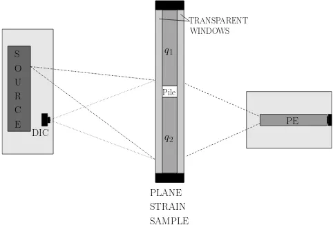
PLANE STRAIN SAMPLE S
O U R C
E PE
DIC
Pile
TRANSPARENT WINDOWS
q2
q1
Fig. 2. Schematized plan view of PE model test setup; laser source, plane strain sample, and photoelastic acquisi-tion.
4 Example: pile in granular medium
The newly developed polariscope was mainly developed to study the stress and strain behaviour in plane strain physical models in which the non-cohesive soil (like sand) is substituted by broken glass. An example setup studies pile installation. A square model pile with a surface area of 16 x 20 mm2is pushed into a plane strain strongbox with inner dimensions 400 x 400 x 21 mm3. The box is filled with broken glass. After each 1 mm increment a photoelastic measurement is made and an additional photo is taken for the digital image correlation. Meanwhile the forces on the pile head and of the surcharge load on the surface level are monitored.
4.1 Setup
The setup, as sketched in plan view in Fig. 2, can be divided in three parts. The source of the polarized light, and the camera for the digital image correlation (DIC) are located at one side of the sample. The light source is offset from the center line of the sample to reduce reflections and glare effects that interfere with the measurements. The sample is contained in a glass and steel strongbox and loaded with two surcharges q1and q2. The pile is centered in the strongbox. On the other side of the sample the remaining components of the photoelastic (PE) setup are situated. As seen in the sketch only about half of the sample is within the field of vision of the cameras. The pile is completely in the view, but only half of the soil surrounding the pile. This improves the spatial resolution of the DIC and PE analysis, as less surface area is covered with the fixed resolution of the camera.
The two retardation plates and the analyser are mounted in a computer controlled rotational stage. A standard prosumer DSLR camera was used for the image acquisition for the DIC and the PE mea-surements. These camera were also remotely controlled. All polarisation optics were sourced from Newport and 2” in diameter.
4.2 Results
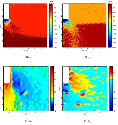
The resulting stress and strain fields after 40 mm of pile installation are shown in Figs. 3(a) and 3(b) for the stress stateσxx andσyy. These plots show the full pile width, but only one side of the soil surrounding the pile. The scale is normalized on this full pile width. The total height and width is seven times the pile width. For a similar region the horizontal and vertical strains are plottedεxxand
x/W (−)
y/W (−)
1 2 3 4 5 6
1 2 3 4 5 6 −2000 −1800 −1600 −1400 −1200 −1000 −800 −600 −400 −200 0 [kPa]
(a)σxx
x/W (−)
y/W (−)
1 2 3 4 5 6
1 2 3 4 5 6 −2000 −1800 −1600 −1400 −1200 −1000 −800 −600 −400 −200 0 [kPa]
(b)σyy
x/W
y/W
1 2 3 4 5 6
1 2 3 4 5 6 −0.4 −0.2 0 0.2 0.4 0.6 0.8 1
(c)εxx
x/W
y/W
1 2 3 4 5 6
1 2 3 4 5 6 −1 −0.8 −0.6 −0.4 −0.2 0 0.2
(d)εyy
Fig. 3. Horizontal and vertical stressesσxx&σyyand strainsεxx&εyyafter 40 mm of pile displacement, negative sign is compressive,contractive.
Clearly, reasonable values for the stress are only found in the high stress zones near the pile where the retardation angle is sufficiently high. In the lower half of theσxx-plot positive values are found. With exception of some outliers the results for the vertical stressσyyare all compressive.
5 Conclusions
The current paper re-introduces the photoelastic measurement method in experimental geomechanics. A full-field phase stepping polariscope suitable for geomechanics has been developed. Additionally, the setup facilitates a second camera for digital image correlation. Together the setup potentially offers new insight in the strain and stress paths in (geomechanical) physical model tests.
As example a pile installation problem is shown for which both the strain and the stress fields for 40 mm of pile installation are presented.
References
1. M.M. Frocht, Photoelasticity Volume 1 (John Wiley & Sons, New York, 1946)
2. P. Dantu, Proceedings of the Fourth International Conference on Soil Mechanics and Foundation Engineering, (1957), 144–148
3. A. Drescher, G´eotechnique, 264, (1976), 591–601.
4. T., Wakabayashi, Proceedings of the seventh Japanese National Conference on Applied Mechanics, (1957), 153–158
5. A. Ajovalasit, S. Barone, G. Petrucci, Journal of Strain Analysis, 332, (1998), 75–91 6. H.G.B. Allersma, Experimental Mechanics, 229, (1982), 336–341
7. M.R. Dyer, Observation of the stress distribution in crushed glass with applications to soil rein-forcement, (PhD thesis, University of Oxford, 1985)
8. M. Da Silva, J. Rajchenback, Nature, 4066797, (2000), 708–710 9. D.W. Howell, R.P. Behringer, C.T. Veje, Chaos, 93, (1999), 559 – 572
10. D. J. White, W.A. Take, M.D. Bolton, Proc. of the 10th Int. Conf. on Comp. Meth. and Advances in Geom. Tucson, Arizona, (2001), 997–1002
11. J. Dijkstra, On the Modelling of Pile Installation, (PhD thesis, Delft University of Technology, 2009)
12. S. Yoneyama, H. Kikuta, Experimental Mechanics, 463, (2006), 89–296
13. J.W., Dally, W.F. Riley, Experimental Stress Analysis Third Edition (McGraw-Hill, Singapore, 1991)
14. D.C. Ghiglia, M.D. Pritt, Two-Dimensional Phase Unwrapping, (John Wiley & Sons, Inc., New York, 1998)