ABSTRACT
LIN, CHUAN. Heavy Traffic and Markov Modulated Models for Wireless Queueing Sys-tems and Numerical Methods for Associated Resource Allocation Problems. (Under the direction of Robert Buche.)
This dissertation is concerned with heavy traffic and Markov modulated diffusion mod-els that are applied to resource allocation problems in wireless communication system and the numerical analysis for their associated continuous time stochastic control problems. To be specific, the heavy traffic model is a two-dimensional stochastic differential equation with reflection (SDER), and the other model is a second-order Markov modulated diffusion process.
communities.
transmission power as well as maintain acceptable levels for the SINR.
HEAVY TRAFFIC AND MARKOV MODULATED
MODELS FOR WIRELESS QUEUEING SYSTEMS AND
NUMERICAL METHODS FOR ASSOCIATED RESOURCE
ALLOCATION PROBLEMS
BY
CHUANLIN
A DISSERTATION SUBMITTED TO THE GRADUATE FACULTY OF
NORTH CAROLINA STATE UNIVERSITY
IN PARTIAL FULFILLMENT OF THE
REQUIREMENTS FOR THE DEGREE OF
DOCTOR OF PHILOSOPHY
OPERATIONS RESEARCH-MATHEMATICS
RALEIGH, NORTH CAROLINA
DECEMBER, 2006
APPROVED BY:
TAOPANG KAZUFUMIITO
ROBERTBUCHE HIENTRAN
Biography
Chuan Lin was born on Oct. 20th, 1976 in Chongqing city, P.R.China. After he finished his high school education in September, 1995 at famous Nankai Middle School in Chongqing, Sichuan province, he entered University of Science and Technology of China (USTC) in Hefei, Anhui province.
From 1995-2002, he earned his B.S degree in mathematics and M.S. degree in Oper-ations Research at USTC. In 2002, he got an offer from North Carolina State University and began his new life in United States. At NCSU, he studied for his PhD degree in Oper-ations Research and worked with professor Robert Buche on stochastic control problem in wireless communication system and graduated at Dec. 2006.
Acknowledgments
I am very grateful to my advisor, Professor Robert Buche, for introducing me the heavy traffic approach and its application in the engineering fields. For me, he’s not only my advisor, but also the colleague and friend. I remember four years ago, I knew nothing about probability theory and stochastic calculus, he introduced me those concepts and encouraged me take the advanced theoretic courses. I remember that he provided various opportunities to me to attend related seminars, workshops and conferences, to communicate and study from the pioneers of these fields, these activities broadened my eyes and were invaluable for my research. I was realizing that probability and stochastic process theories are valuable tools in the real world. I still remember that when I worked with him on the ARO (Army Research Office) projects, he taught me how to handle a large project step by step, I think that experience is important for me in the past, present and in the future. I am also grateful for his input for making my dissertation better. I really appreciate his help on my thesis writing, it is very useful for me, whose native language is not English.
I would like to thank Operations Research program in NC State University; this inter-disciplinary program is very flexible and provides students lots of chances to choose what they would like to do in their research area and their future career. Also I thank OR program for providing me the first two year financial support.
I thank the Mathematics Department to give me opportunity to be a lecture assistant for three semesters, it provided me financial support, and most importantly, the teaching experience was enjoyable and valuable for my future career.
great opportunities to cooperate with industry people.
Although most people helped me along the way, none is more responsible for my com-pleting my dissertation than my girlfriend, Jing Gao. When I was frustrated and upset, she always stayed with me, supported me, shared my pain and my pleasure. Staying around her I feel I am becoming a better person.
Table of Contents
List of Tables vii
List of Figures viii
1 Heavy Traffic Modeling in Wireless Communication Systems 1
1.1 Introduction and Motivation . . . 1
1.2 Basic Model . . . 4
1.2.1 Mean Rate and Balance Equation . . . 4
1.2.2 Scaling and Dynamic System Equation . . . 7
1.3 The Reflection Processzn(·) . . . 13
1.3.1 Overview of SDER . . . 13
1.3.2 Basic Definition . . . 14
1.3.3 Multi-CompletelyS . . . 18
1.4 The Control Problem . . . 23
2 Numerical Methods for Continuous-Time Stochastic Control Problems 26 2.1 Overview and Introduction of Markov Chain Approximation Method . . . . 26
2.2 Construction of Approximation Markov Chain . . . 29
2.2.1 Stochastic Control Problem . . . 29
2.2.2 Transition Probability and Local Consistency inG0 . . . 31
2.2.3 Approximation for Reflecting Boundaries∂G . . . 35
2.3 Dynamic Programming Equation and Computational Methods . . . 41
3 Numerical Experiments and Real Time Simulations 46 3.1 Introduction and Simulation Design . . . 46
3.2 Policy Generation Simulation . . . 50
3.2.1 Channel Condition . . . 50
3.2.2 Weight and Cost . . . 54
3.2.4 Grid Size . . . 71
3.3 Simulation . . . 74
3.3.1 Monte Carlo Simulation . . . 76
3.3.2 Poisson Arrival Process . . . 80
3.3.3 Tele-Traffic Models . . . 85
4 Markov Modulated Model for Wireless Queueing Systems 103 4.1 Introduction and Motivation . . . 103
4.2 Problem Statement . . . 104
4.3 Stochastic Control Problem and Numerical Analysis . . . 109
4.3.1 Value function and the HJB equation . . . 109
4.3.2 Numerical Method for Markov Modulated Stochastic Control Prob-lem . . . 111
List of Tables
List of Figures
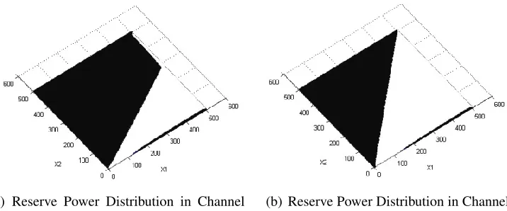
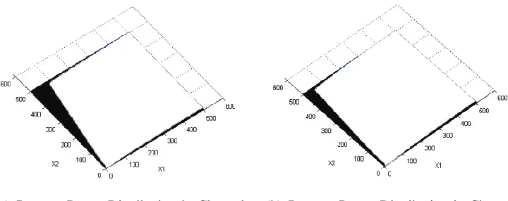
Figure 1.1 Illustration of One Cell System . . . 5 Figure 2.1 Illustration of uniformh-Grid . . . 38 Figure 2.2 Simple illustration ofMulti-CompletelyS in two Dimensional case . 39 Figure 2.3 Approximating Reflection Directions on the Boundary . . . 40 Figure 2.4 Simple Example of Approximating Chain on Boundary . . . 40 Figure 3.1 Illustration of Control (Reserve power) Distribution . . . 50 Figure 3.2 Power Distribution in Queue 1, λ¯ = (0.08,0.1; 0.1,0.08), π =
(0.5,0.5) . . . 52 Figure 3.3 Power Distribution in Queue 2, λ¯ = (0.08,0.1; 0.1,0.08), π =
(0.5,0.5) . . . 52 Figure 3.4 Power Distribution in Queue 1, λ¯ = (0.08,0.1; 0.1,0.08), π =
(0.8,0.2) . . . 53 Figure 3.5 Power Distribution in Queue 2, λ = (0.08,0.1; 0.1,0.08), π =
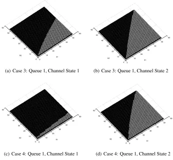
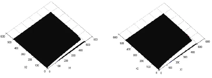
(0.8,0.2) . . . 54 Figure 3.6 Power Distribution in Queue 1 ofCase 3 & 4 . . . 55 Figure 3.7 Power Distribution in Queue 2, λ¯ = (0.08,0.1; 0.1,0.08), π =
(0.8,0.2) . . . 56 Figure 3.8 Power Distribution in Queue 1 at Channel State 1 for Difference
weightC1 . . . 57
Figure 3.9 Power Distribution in Queue 1 at Channel State 2 for Difference weightC1 . . . 58
Figure 3.10 Power Distribution in Queue 1 whenp1 = 3&p2 = 2 . . . 59
Figure 3.11 Illustration of Combined Reflection Directions on Different Channel States . . . 61 Figure 3.12 CompletelySfor reflection process of Case 1 & 3 . . . 62
Figure 3.16 Effect of Reflection Process on Queue 1&2 at Channel state 2,λ =
(0.06,0.08; 0.1,0.08) . . . 66
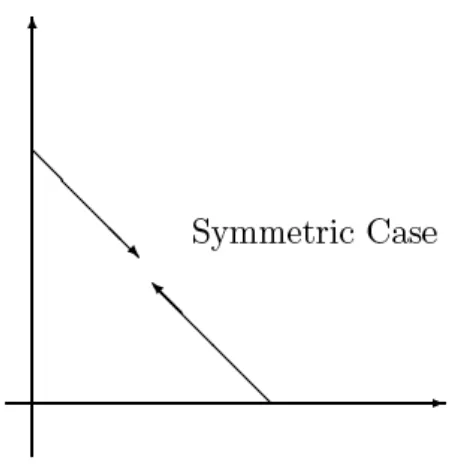
Figure 3.17 NonCompletelyS in a Symmetric Reflection Process . . . 67
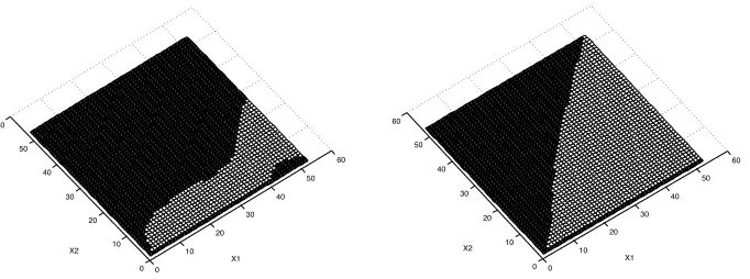
Figure 3.18 Effect of Reflection Process (NonCompletelyS ) of Control Policy on Queue 1,λ= (0.06,0.08; 0.1,0.08) . . . 68
Figure 3.19 Illustration ofMulti-CompletelyS . . . 69
Figure 3.20 Optimal Control Policy of Queue 1 when reflection Process is Multi-CompletelyS ,λ= (0.06,0.08; 0.1,0.08) . . . 70
Figure 3.21 Non Completely S condition Control Policy at Channel State 1 (Cunderf low = 10, Coverf low = 250) . . . 71
Figure 3.22 Control Policy in non-Completely S condition, Cunderf low = 30, ‘Coverf low = 250,λ= (0.06,0.08; 0.1,0.08) . . . 72
Figure 3.23 Power Distribution of Queue 1,B = 5, h= 0.1 . . . 73
Figure 3.24 Power Distribution of Queue 1,B = 5, h= 0.05 . . . 73
Figure 3.25 Power Distribution of Queue 1,B = 5, h= 0.025 . . . 74
Figure 3.26 Power Distribution of Scenario 1 in Table 3.4 . . . 75
Figure 3.27 Power Distribution of Scenario 2 in Table 3.4 . . . 76
Figure 3.28 Power Distribution of Scenario 3 in Table 3.4 . . . 77
Figure 3.29 Monte Carlo: Queue One Evolution,C1 =C2 = 1, p1 =p2 = 2 . . . 78
Figure 3.30 Monte Carlo: Queue Two Evolution,C1 =C2 = 1, p1 =p2 = 2 . . 79
Figure 3.31 Monte Carlo: Queue One Evolution,C1 = 10, C2 = 1, p1 =p2 = 2 . 80 Figure 3.32 Monte Carlo: Queue Two Evolution,C1 = 10, C2 = 1, p1 =p2 = 2 . 81 Figure 3.33 Monte Carlo: Queue One Evolution,C1 =C2 = 1, p1 = 2, p2 = 3 . 82 Figure 3.34 Monte Carlo: Queue Two Evolution,C1 =C2 = 1, p1 = 2, p2 = 3 . 83 Figure 3.35 Poisson Arrival: Queue One Evolution,C1 =C2 = 1, p1 =p2 = 2 . 84 Figure 3.36 Poisson Arrival: Queue Two Evolution,C1 =C2 = 1, p1 =p2 = 2 . 85 Figure 3.37 Poisson Arrival: Queue One Evolution, C1 = 10, C2 = 1, p1 = p2 = 2 . . . 86
Figure 3.38 Poisson Arrival: Queue Two Evolution, C1 = 10, C2 = 1, p1 = p2 = 2 . . . 87
Figure 3.39 Poisson Arrival: Queue One Evolution,C1 =C2 = 1, p1 = 2, p2 = 3 88 Figure 3.40 Poisson Arrival: Queue Two Evolution,C1 =C2 = 1, p1 = 2, p2 = 3 89 Figure 3.41 Batch Poisson Arrival Process . . . 92
Figure 3.42 Batch Arrival: Queue One Evolution,C1 =C2 = 1, p1 =p2 = 2 . . 93
Figure 3.43 Batch Arrival: Queue Two Evolution,C1 =C2 = 1, p1 =p2 = 2 . . 94
Figure 3.49 Aggregated ON/OFF Traffic,N = 20 . . . 99 Figure 3.50 ON/OFF: Queue One Evolution,C1 =C2 = 1, p1 =p2 = 2 . . . 99
Figure 3.51 ON/OFF: Queue Two Evolution,C1 =C2 = 1, p1 =p2 = 2 . . . 100
Figure 3.52 ON/OFF: Queue One Evolution,C1 = 10, C2 = 1, p1 =p2 = 2 . . . 100
Figure 3.53 ON/OFF: Queue Two Evolution whenC1 = 10, C2 = 1, p1 =p2 = 2 101
Figure 3.54 ON/OFF: Queue One Evolution,C1 =C2 = 1, p1 = 2, p2 = 3 . . . 101
Figure 3.55 ON/OFF: Queue Two Evolution,C1 =C2 = 1, p1 = 2, p2 = 3 . . . 102
Chapter 1
Heavy Traffic Modeling in Wireless
Communication Systems
1.1
Introduction and Motivation
to a more general queue network. The modern approach to queue networks was initiated by Reiman [69], in which he proved a heavy traffic limit theory for single class network. Following this, there was an explosion of interest in networks, including single class and multiclass. A survey of work on queue networks is in [86].
Basically, three aspects of advantages on the heavy traffic approach are desirable, first, compared with the original physical system, which is usually not mathematical tractable, the structure of the limit equation for the queue dynamics becomes much simpler - it only contains the first and second moment information of the arrival and service processes for the real system, other finer details disappear. Secondly, even though we are considering a sequence of queueing system instead of a single one, the limit diffusion process provides a good approximation for the quantities of interest, such as stationary mean and variance, even if the system is under heavy traffic; another advantage is we can use numerical method to solve the system. For example, if the limit equation is happened to be a controlled diffusion process, then the Markov Chain(MC) approximation method [52] can be used, this numerical method for heavy traffic analysis of controlled queueing system is one of the main parts of our thesis.
• With the proliferation of wireless applications having large capacity require-ments, such as multimedia, internet, gaming, etc., and the limitations of real-izing spectral efficiency gains, wireless communication systems will be oper-ating an near capacity levels. In this regime efficient resource allocation has paramount importance and heavy traffic methods (which, loosely speaking, assume the system is operating at near-capacity) is an natural setting for the resource allocation problem;
• Compared with wireline queueing systems whose service rate is determined in general, the mobile system involves much more technical details and chal-lenges. Due to multiple time scales, fast and slow fading, link loss, and wide bandwidth, etc., the wireless system can switch between various service modes at different times, while the customers receive service at rates that depend ex-clusively on the particular mode the system is in at each point in time. Never-theless, despite the contrast to wireline system, in heavy traffic analysis point of view, they share the analogous benefits. In other words, through appropriate scaling, the use of an averaging or asymptotic method (heavy traffic approxi-mation) still seems to be desirable;
• Channel condition measurement is possible in the real wireless queueing sys-tem, for example, the report in [7] develops a system that is designed for time-varying channels and allows the test signals (pilot) to control or measure the channel condition. As a result, we can suppose the statistics of channel condi-tion is observable;
• Finally, the comprehensive exposition of heavy traffic method in queueing sys-tem and numerical method [52] for stochastic control problem provide us rich theory and powerful tools to explore the optimal policies for the underlying control problem.
heavy traffic analysis into mobile queueing system. In their model, the total power of base station is divided into two parts, one is the nominal power to handle the mean arrival rate, the other is reserve power, which is very small compared with nominal power and can be allocated at will to control the queue fluctuation. As usual in heavy traffic analysis, the real system is imbedded in a sequence of system with parameter n, as n → ∞, the transmitter idle time goes to zero, however, one applies a scaling dependent on the channel process to get the limit dynamics, under an assumption on the reflection process, namely the completely-Scondition. The limit process turns out to be a stochastic differential equation with reflection (SDER), which eliminates inessential detail since much useful qualitative information can be read off from the scalings and the form of the (controlled) drift term and Wiener process covariance. The stochastic control problem in [14] is to determine how to allocatereservepower to optimize some performance criterion. Nevertheless, an analytical solution for stochastic control problem is hard to obtain in general, only some intuition for stochastic control problem are given in [14]. In [13], the numerical method for continuous time stochastic control problem (see [52]) is introduced to get the optimal policies for the reserve power. Our initial simulation shows that the optimal policy has a Max Weight structure [75] and the reflection process is seen to influence its form. Furthermore, we found that the optimal policies are also affected by many variables, such as channel process, parameter of cost function, heavy traffic condition, etc, furthermore, we will take a closer look at the reflection process too. The real time queueing system using our optimal policies compared with some heuristic policy is still worth to be investigated. The first part of this thesis is an full expansion of [13] and systematic study towards this goal.
1.2
Basic Model
1.2.1
Mean Rate and Balance Equation
via randomly time-varying channels. Data, destined for the various individual remote units and measured in packets, arrives at the base station according to some random process, and is queued according to its destination.
8T 8T 8T 8+T
MOBILE
MOBILE
MOBILE
MOBILE+
/NE#ELL3YSTEM
Data Arrivals
!T !T !T !+T
Vector Channel State Process
L(t) = j
P + u
$+T
$T
$T $T
Figure 1.1: Illustration of One Cell System
The individual random channel variations might be correlated. We are concerned with the assignment of power to the various queues on the forward link as well as understanding the dependencies of the queue process on the parameters and driving processes. Letj = 1, . . . , J denote the possible states of the set of K channels: Each value of j specifies the states of all of the channels in a vector withK components. Under the assumption of heavy traffic, we divide the total power in the base station into two parts: one is the nominal power to handle the ”mean” loads, and the other small part, which depends on the queue and channel states, is ”reserve” power (control) to handle the stochastic variations of queue processes.
As usual in the heavy traffic analysis, we embed the real system into a family of queue-ing system parameterized by index n. For the parameter n, let An
i(t) define the arrival process for queue i, whose mean data arrival rate isn¯λa
O(n). Recall that the new feature of wireless queueing system is time-varying channels, which is usually modeled as the continuous time Markov chain with finite state, see [83,90]. Similarly, we defineLn(t) = L(nνt), ν ∈ (0,1) be thevector channel process. Its state is characterized by indexj ∈ J, each j specifies the channel for allK mobiles. In our case, we suppose thatj specifies a vectorλ(j) = λd1(j), λd2(j), . . . , λdK(j) , the achiev-able transmission rate/unit power, where j evolves according to a semi-Markov process andLn(t)has a stationary distributionπ(j)due to the assumption that the channel process is a continuous time Markov chain (CTMC). It is important to note that the channel process varies at a rateO(nν)which is slower than that of the arrival processO(n), we think this assumption is reasonable since in practical world, the channel is often in the same state over many arrivals and departures. The third related process is departure process Dni(t), recall the nominal powerp¯which is split from the total power of the base station to handle the mean arrival rate of data, thus, for parameter n, the mean departure rate for queueiis given by averaging over the channel stationary distributionπ, thus, the mean arrival rate to queueiequals the average service rate
¯
λaiv¯bi = Λai ≈X j∈J
λdi(j)¯pi(j)π(j) (1.2.1)
Another part of power split from the base station is u >¯ 0, we supppose that the total reserve power level is u/n¯ ν/2, and this is split among the queues, i.e., there are such that
P
preallocate the nominal power and reserve power, is there any tradeoff between them? We won’t focus this question here, interested readers can refer [25], which contains several models to analyze power preallocation.
1.2.2
Scaling and Dynamic System Equation
In order to establish the heavy traffic stochastic process limits, the general idea is to repre-sent the queueing ”content” process of interest as a reflection of a corresponding net-input process. It turns our that the scaled net-input process involves convergence toWiener pro-cess due to the application of (functional) central limit theory, and the limit process for the queueing processes is reflected diffusion process. The main difference of the queueing process in wireless system from that in wireline is time-varying channels, which randomly produce various service modes at each time instant, thus it is desirable that the scaled net-input process can show the effect of channel evolution. As a consequence, the scaling is determined by the channel state process, not by the arrival or service processes contrary to the usual situation in heavy traffic analysis. Under this scaling system, the service and data arrival terms will be represented in a form that suggests the limit process. Recall that the channel processes change at rateO(nν), ν ∈(0,1), defineγ = 1−ν/2, Letxn
i(t)be1/nγ times the content of queue i, and let the arrival process An
i(t) be1/nγ times the number that have arrived. When a queue is empty, its power might be reassigned. LetDin(t)denote
1/nγ times the number of packets that were sent from queuei byt, but not including the packets sent with power reallocated to queue because another queue was empty, also letyn
ki denote1/nγ times the number of packets that have been sent from queue with the part of the power levelsp¯k(j), j ≤ J, that were reassigned from queuek toiwhenk was empty. Simply, the content of queue process is given by:
xni(t) = xni(0) +Ain(t)−Din(t)−X k
ykin(t) (1.2.2)
(i). The Arrival Process:
• Consider the simplest case, i.e., the fluid arrival model. From (1.2.1), the scaled arrival process is given by:
Ani(t) = n
nγΛ a it=
1
nν/2n
ν
Λait (1.2.3)
Hence, we can say that the scalings for time and space arenν andnν/2 re-spectively, which correspond to the changing rate or dynamics of channel process. We will see this later in the discussion of departure process and reflection term.
• Now, let’s move on a more general and unrestrictive arrival model. Let
Sia,n(t)be1/ntimes the number of packets that have arrived to queueiby timet. Define ∆a,ni,l to be the lth interarrival interval for queuei. λ¯a
i and
¯
vibdenote the mean packet arrival rate and packet size. Thus, the constant
¯ ∆a
i = 1/λ¯ai is defined to be mean interarrival interval for the batches and
vb
i,l is packet size forlth batch arriving the base station. Then, the arrival process can be written as
Ani(t) = 1
nγ nSa,ni
X
l=1
vi,lb
= 1
nγ
nSa,ni (t)
X
l=1
[vi,lb −v¯ib] + v¯
b i
nγ
nSia,n(t)
X
l=1
1−∆ a,n i,l ¯ ∆a i
+ ¯v
b i
¯ ∆a
inγ
nSia,n(t)
X
l=1
∆a,ni,l
=Mia,n(t) + v¯
b i
¯ ∆a
inγ
nSia,n(t)
X
l=1
∆a,ni,l
=Mia,nj(t) + v¯
b i
¯ ∆a
inγ
(nt−un(t))
where
Mia,n(t) = 1
nγ
nSa,ni (t)
X
l=1
[vi,lb −¯vib] + v¯
b i
nγ
nSia,n(t)
X
l=1
1−∆ a,n i,l ¯ ∆a i
and un(t) is and “error”, which is nt minus the time of the last arrival before or at nt. Thus, 1/∆¯ainγ times this error is a residual-time error term. Hence,
Ani(t) =Mia,n(t) + n
nγΛ a it−
n(t) (1.2.5) wheren(t) = ¯vb
iun(t)/∆¯ainγ. Later we will show thatM a,n
i (t)andn(t) converge to0in distribution, then (1.2.5) is same as (1.2.3) in fluid model.
(ii). The Departure ProcessDn
i(t): From the discussion of previous section, we can write
Dni(t) = n
nγ
Z t
0
X
j∈J
I{Ln(s)=j}¯λdi(j)
×
¯
pi(j) +
ui(j, xn(t)
nν/2
×I{xn
i(s)>0}ds
(1.2.6)
DroppingIxn
i(s)>0, thenominalmean departure rate for queueiis
Di0,n(t) = n
nγ
Z t
0
X
j
I{Ln(s)=j}¯λdi(j)¯pi(j)ds (1.2.7)
Then we define the scaled idle time terms for queueiin channel statej as follows:
Tin(j, t) = n
nγ
Z t
0
I{Ln(s)=j}I
{xn
i(s)=0}ds (1.2.8)
thus, the total scaled idle time isTin(t) = P
jT n
i (j, t). Let
yin(t) = X
j
¯
Intuitively, yin(t) is the (scaled) number that could have been transmitted fromi at times s ∈ [0, t]when xn
i(s) = 0 with the allocations p¯i(j), j ∈ J, had there been packets to transmit. Therefore, rewriteDn
i(t)as:
Din(t) = Di0,n−yni(t) +
Z t
0
X
j∈J
¯
λdi(j)ui(j, xn(s))I{Ln(s)=j}ds (1.2.9)
When one of the queues is empty, our policy is to redistribute its nominal power to other nonempty queues so as to utilize the resource as much as possible. Letpki(j) denote the part ofp¯k(j)redistributed from an empty queue k to queuei in channel statej. Define
ynki(j, t) = ¯λdi(j)pki(j)Tkn(j, t)
the (scaled) number from queueitransmitted on[0, t]due to the power reallocations from an empty queuekto queuei, when the channel state isj, then
ykin =X
j∈J
ykin(j, t)
The value ofpki(j)depends on the policy when a queue is empty.
Then, combine (1.2.5) and (1.2.9), (1.2.2) is expanded to
xni(t) = xin(0) +Mia,n(t) + n
ν
nν/2Λ
a it−D
0,n
i (t) +z n i(t) −
Z t
0
X
j∈J
I{Ln(s)=j}λ¯di(j)ui(j, xn(s))ds+n(t),
zin(t) = yin(t)− X j,k6=i
ynki(j, t)
(1.2.10)
to the heavy traffice condition (1.2.1) , define
Mid,n(t) = n
ν
nν/2Λ
a it−
n nγ Z t 0 X j
I{Ln(s)=j}λ¯di(j)¯pi(j)ds
= n
ν
nν/2
X
j∈J
¯
λdi(j)¯pi(j)−
nν nν/2
Z t
0
X
j
I{Ln(s)=j}λ¯di(j)¯pi(j)ds
= 1
nν/2
Z tnν
0
X
j
πj−I{L(s)=j}
¯
λdi(j)¯pi(j)ds
(1.2.11)
where the heavy traffic condition was used in 1.2.11, we can now write (1.2.10) as
xin(t) =xni(0) +Mia,n(t) +Mid,n(t)
−
Z t
0
X
j∈J
I{Ln(s)=j}¯λdi(j)ui(j, xn(s))ds+n(t),
zin(t) =yni(t)− X j,k6=i
ykin(j, t)
(1.2.12)
We state the fundamental convergence theorem (Theorem 5.1 in [14]) for (1.2.10) with-out proof as follows:
Theorem 1.2.1 Letui(j, x)be measurable function ofxthat are continuous almost every-where with respect to Lebesgue measure. Letxn(0) ⇒ x(0). Then Ma,n(·) ⇒ 0, i ≤ K, andMd,n(·)converges weakly to a Wiener processw(·) = {wi(·), i≤K}with covariance
aik =Ewi(1)wk(1) = 2E
" X
j
I{L(0)=j}λ¯di(j)¯pi(j)−Λai
# × Z ∞ 0 " X j
I{L(τ)=j}λ¯dk(j)¯pk(j)−Λak
#
dτ
(1.2.13)
mutually independent. Also
(xni(·),Mid,n(·), Tin(j,·), yin(·), yi,kn (·);i, k ≤K, j ≤J)
⇒(xi(·), wi(·), Ti(j,·), yi(·), yik(·);i, k ≤K, j ≤J) which satisfies
xi(t) = xi(0) +
Z t
0
bi(u, x(s))ds+wi(t) +zi(t) (1.2.14) wherebi(u, x) =−
P
j¯λ d
i(j)ui(j, x)Π(j)and
zi(t) = yi(t)−
X
k6=i
yki(t) (1.2.15)
yi(·)andyik(·)can increase only whenxi(t) = 0where
yi(t) =
X
j
¯
λdi(j)¯pi(j)Ti(j, t)
yik(t) =
X
j
¯
λdk(j)pik(j)Ti(j, t)
X
k6=i
pik(j)≤p¯i(j)
The state space for the scaled queue is the positive orthantRK
1.3
The Reflection Process
z
n(·)
1.3.1
Overview of SDER
In the previous section, we have shown that (1.2.10) weakly converges to a process satisfy-ing stochastic differential equation with reflection (SDER) as follows:
xi(t) = xi(0) +
Z t
0
bi(u, x(s))ds+wi(t) +zi(t) (1.3.1)
where bi(u, x) = −
P
jλ¯ d
i(j)ui(j, x)Π(j). The basic questions are the existence and uniqueness of such processes like (1.3.1), i.e., the diffusion processes with boundary con-ditions (smooth or non-smooth domains), chiefly with instantaneous reflection. Actually, these topics have been studied by many authors since 1960s’. Skorokhod [73], Watan-abe [84], Stroock and Varadhan [76], just to mention a few here, deal with processes in
R1, or in smooth domains ofRn, with smooth boundary conditions. However, models ap-pearing in some application fields, mainly led by heavy traffic analysis in queueing theory, require us to consider the diffusion process in non-smooth boundary conditions (see for in-stance, Reiman [69], Harrison and Williams [35]). Harrison and Reiman [34], Reiman and Williams [70] discuss the existence and uniqueness from the heuristic and practical point of view, in their case, the domain for diffusion process is multidimensional nonnegative orthantRd
+. Dupuis and Ishii [23] [24], and Lions and Sznitman [57] investigate this
prob-lem in a more general domain and reflection condition. Almost all of the aforementioned authors use the idea calledSkorokhod Problem approach[20] (defined at the following sec-tion), i.e. they consider the properties of reflection mapping:C[R+, Rd]→C[R+, Rd]and
prove the existence and uniqueness of Skorokhod Problem, whereC[R+, Rd]is the
contin-uous functional space in[R+, Rd]. As well as we know, the most general result is given by
Dupuis and Ishii [23] [24], they show that when the reflection mapping is Lipschitz con-tinuous on a subset ofC(R+, Rd)that contains all functions with bounded variation, there
On the other hand, the conditions in [23] [24] are hard to verify and not very practi-cal. The models in [34, 70], which arise directly from queueing theory, posed the prob-lem of stochastic processes with boundary conditions in nonsmooth domains, for instance with edges and corners. In [70], Reiman and Williams claimed an importantComplete-S property for the reflecting matrix. This property is shown to be the necessary [70] and sufficient [80] for the existence of the solution for the SDER, especially, such property is equivalent to the conditions in [23].
Our discussion of SDER is mainly from the practical side, furthermore, we think the CompletelyS condition, which is discussed heavily in Buche & Kushner [14], simplifies the reflection process. In most of the discussion, they consider the reflection direction statically as if the queue always empties in a unique channel state. However, the “server system” for each queue is always changing, i.e., the departure rate is switching from one level in a particular channel state to another. So can theCompletelyScondition for wireline system still be applied to the mobile queue system with time-varying channel state? Is it too strong? How the system manager reallocate the extra nominal power when one queue is empty at each channel state? In this thesis, we propose a new condition, which is weaker than CompletelyS condition so calledMulti-Completely S , and show that it is indeed a necessary condition for the existence of our limitingStochastic Differential Equation with Reflection.
1.3.2
Basic Definition
In order to study (1.3.1) in a more general framework, we would like to introduce the standard approach for SDER orReflected diffusion, theSkorokhod Problem. The following material is specialized to the cases of interest of this thesis.
then it is referred as acorner.
Definition 1.3.1 (Skorokhod Problem) Letz(·)be anRn-valued function of bounded vari-ation on each time interval. C([0, T],Rn) be the continuous mapping from[0, T]to Rn. Letψ(·)∈ C([0, T],Rn)withψ(0) ∈ G. Then we say thatx(·), z(·)solves the Skorokhod Problem forψ(·)if
(i). x(t) =ψ(t) +z(t), x(0) =ψ(0)
(ii). x(t)∈Gfort∈[0, T]
(iii). |z|(T)<∞, where|z|(t)denotes its total variation over[0, T]. (iv). |z|(t) =R0tI{x(s)∈∂G}d|z|(s)
(v). There exists measurable function γ : [0, T] → Rn such that γ(t) is in the positive convex cone generated byd(x(t))andz(t) = R0tγ(s)d|z|(s).
The last condition can be alternatively written as
z(t) = X
i
yi(t)di (1.3.2)
whereyi(0) = 0andyi(·)is nondecreasing and can increase only att wherex(t) ∈∂Gi. (1.3.2) is similar with the reflection limiting result, see (1.2.15) in our wireless model.
In Skorokhod Problem framework, we can discuss the existence and uniqueness of Stochastic Differential Equation with Reflection (SDER). Let (ω,F, P) be the probabil-ity space,{Ft, t≥0}a filtration, and w(·)anFt standard vector-valued Wiener process. If the control variable is non-anticipative with respect tow(·), we then say thatu(·)is an admissible control with respect to w(·). Then an Ft-adapted process x(·)is a solution to the reflected stochastic differential equation for initial conditionx(0)if it solves
x(t) =x(0) +
Z t
0
b(x(s), u(s))ds+
Z t
0
where
|z|(t) =
Z t
0
I{x(s)∈∂G}d|z|(s)<∞
and where there exists anFt adapted process γ(·)with γ(s) taking values in d(x(s))for almost all(w, s)and such that
z(t) =
Z t
0
γ(s)d|z|(s).
Thus,(x(·), z(·))solves the Skorokhod problem for
ψ(t) =x(0) +
Z t
0
b(x(s), u(s))ds+
Z t
0
σ(x(s))dw(s).
After defining the solution for SDER, the remaining question is to find the conditions under which there exists a unique solution for (1.3.3). Rewrite (1.3.3) with reflection (1.3.2) as a compact form as following:
X(t) = Φ(t) +RY(t)⇒dX(t) =dΦ(t) +RdY(t) (1.3.4)
whereΦ(t)is an n-dimensional diffusion process in state spaceGwith drift vectorb and covariance matrixΓ = (σij),Y(t)is an×1non-decreasing vector process, and increases only whenΦ(t)hits the boundary∂G,R is called as the reflection matrix. Due to Reiman and Williams [70],Complete-S plays an crucial role in the solution existence and unique-ness of SDER (See Theorem 1.3.3):
Definition 1.3.2 (Complete-S) A square matrixAis called Complete-Sif for each princi-pal submatrixA˜ofAthere isy˜≥0such thatA˜y >˜ 0.
property is equivalent to the following. Letl≤K, and consider an arbitraryl-dimensional edge
{x:xi1 = 0, . . . , xil = 0}
of the positive orthant. Letdidenote the reflection direction on
{x:xi = 0, xj >0, j 6=i}
Then there is a vectorv =Pl
j=1ajdij, aj ≥0, starting at the origin ofR
l
+and pointing into
its interior. It seems that theComplete-Scondition is practical, also it is widely recognized in the classical (wireline) queueing network system. We state their theorem as follows without proof, interested readers refer [70](Theorem 2):
Theorem 1.3.3 IfX(t)is a solution of (1.3.4) associated with(b,Γ, R), thenRmust be a Complete-Smatrix.
Also this condition is sufficient for the existence of the solution of (1.3.4) due to [80]. Since our limiting process here is still an SDER, can we assume that the reflection term in (1.3.1) satisfiesComplete-S condition so that it can guarantee the existence and uniqueness of the solution for (1.3.1)? In the next section, we are trying to rewrite our reflection termz(t)in a standard form which is similar with the expression in [34], where the routing matrixRin (1.3.2) equals(I −Q), i.e.,
X(t) = Φ(t) + (I−Q)Y(t). (1.3.5)
1.3.3
Multi-Completely
S
Recall the definitions for idle times and reflection terms in limit processes (1.3.1),zi(·)is known as the reflection term
zi(t) =yi(t)−
X
j,k6=i
yki(j, t). (1.3.6)
whereyi(t) = Pjλ¯di(j)¯pi(j)Ti(j, t)and
Tin(j, t) = n
nγ
Z t
0
I{Ln(s)=j}I{
xn
i(s)=0}ds
= 1
nν/2
Z nνt
0
I{L(s)=j}I{xn
i(s/nν)>0}ds⇒Ti(j, t)
One can treatTin(j, t)as the scaled idle time for queue iin channel statej up to timenνt
asn → ∞, and yi(t)is number of customers that could have been sent usingp¯during the idle time for queuei up to timet, sometimes it is called ”service of fictitious customers”. Additionally, process yi(·)in (1.3.6) is continuous and nondecreasing, yi(0) = 0, and it can increase only at t where xi(t) = 0. Process yki(j, t) is the departures from queue i transmitted on[0, t]due to the power reallocations from an empty queuekto queuei, when the channel state isj, which is
yki(j, t) = ¯λdi(j)pki(j)Tk(j, t)
Suppose we haveKqueuesi= 1, . . . , K andJchannel statesj = 1, . . . , J, then
yi(t) = J
X
j=1
¯
λdi(j)¯pi(j)Ti(j, t)
and
yki(t) = J
X
j=1
¯
λdi(j)pki(j)Tk(j, t)
Then the reflection termzi(t)for queueibecomes
zi(t) = yi(t)−
X
k6=i
yki(t)
that is
zi(t) = J
X
j=1
¯
λdi(j)¯pi(j)Ti(j, t)−
X
k6=i J
X
j=1
¯
λdi(j)pki(j)Tk(j, t)
=
J
X
j=1
¯
λdi(j)¯pi(j)Ti(j, t)− J
X
j=1
X
k6=i
¯
λdi(j)pki(j)Tk(j, t)
= J X j=1 " ¯
λdi(j)¯pi(j)Ti(j, t)−
X
k6=i
¯
λd
i(j)pki(j)
¯
λd
k(j)¯pk(j)
¯
λdk(j)¯pk(j)Tk(j, t)
#
.
(1.3.7)
Let
qki(j) =
¯
λd
i(j)pki(j)
¯
λd
k(j)¯pk(j)
k 6=i
and
Yi(j, t) = ¯λdi(j)¯pi(j)Ti(j, t), i= 1,2, . . . , n.
Due to the property of limiting idle time Ti(j, t), Yi(j, t) is nondecreasing and increases only whenxi(t) = 0and channel state isj. The last line of (1.3.7) can be simplified as:
zi(t) = J
X
j=1
"
Yi(j, t)−
X
k6=i
qki(j)Yk(j, t)
or
Z(t) =
J
X
j=1
(I −QT(j))Y(j, t) (1.3.8)
whereIisn×nidentity matrix andQ(j) = (qki(j))is reflection matrix with zero diagonal elements,Y(j, t)isn×1service of fictitious customersvector. Furthermore, if we define
I = (In×n, . . . , In×n) Q= (QT(1), . . . , QT(J))
whereI andQaren×(nJ)matrix, then
Z(t) = (I − Q)Y(t)
=
I −QT(1)
| {z }
n×n
, I−QT(2)
| {z }
n×n
,· · · , I−QT(J)
| {z }
n×n
Y(t)
(1.3.9)
whereY(t) = [YT(1, t), . . . , YT(J, t)]T, the superscriptT means transpose of matrix. You will see that (1.3.9) has the similar form as the reflection process in (1.3.5). Unfortunately, Complete-S in definition 1.3.2 can not be directly applied on (1.3.9) since Z(t) is the total effect of J different channel states (in other words, various service rate) not only a single service rate in the classical queueing theory. Algebraically, I − Qis not a square matrix, soComplete-S condition in the sense of (1.3.5) can not be applied here. However, due to Fiedler and Ptak [27] (the foundation of Reiman and Williams [70] work), we can still investigate matrices (not necessarily square ones in [70]) which have some positivity properties so calledScondition. Generally speaking, if a matrixAis calledS, there exists a vectory ≥0such thatAy >0. In our case, the compact form of (1.3.1) is
X(t) = Φ(t) + (I − Q)Y(t). (1.3.10) If it has solutions, there exists a nonnegative vectorY(t)such thatZ(t) = (I − Q)Y(t)>
matrix R in (1.3.4) or I − Qin (1.3.5), the reflection term in (1.3.10) will have various reflection direction on the boundary due to not only different reallocation policies (routing) but also channel conditions. Similarly, we can extend the S-condition(positive property) to the principle sub-matrices ofI − Q. When we say the principle sub-matrices ofI − Q, we mean the combination of principle sub matrices (with the identical rows and columns) for each square blocksI −QT(j)(corresponding channel statej) of the rectangle matrix I − Q. Hence, if the principle sub-matrices inherit the positivity properties ofI − Q, we use the same prefix “Multi-completely” to indicate this property. Let’s take an n = 3 -dimensional case as an illustration,
I − Q=
1 q21(1) q31(1)
q12(1) 1 q32(1)
q13(1) q23(1) 1
. . . .
1 q21(J) q31(J)
q12(J) 1 q32(J)
q13(J) q23(J) 1
(1.3.11)
Now the row and column indices of principle matrix of (1.3.11) are both1and3, then the principle matrix is given by
^
I − Q=
"
1 q31(1)
q13(1) 1
!
. . . 1 q31(J) q13(J) 1
!#
(1.3.12)
However, there is some distinction between the Complete-S condition and the Multiple Completely S condition in our case. If there is only one channel state in the wireless communication system, the power reallocation matrix I − Q is a square and Complete-S and Multi-completely S are identical. For multiple channel state, I − Q contains J
(the number of channel state) square blocks, if each square block satisfies Complete-S, I − Qis obviouslyMulti-completelyS, but the reverse is not necessarily true since Multi-completelyS measures the total policy effect in all channel states not a single one. Thus, Multi-completely S is much weaker than Completely S. Sometimes, each square block
communication queueing model. Nevertheless, we still have a similar result as Theorem 2 in [70]:
Theorem 1.3.4 [Multi-completely S] If X(t) is a solution of (1.3.10) associated with
(b,Γ,I − Q), thenI − Qmust be a Multi-CompletelyS matrix.
Proof: LetM =I − Q, supposeM is notMulti-CompletelyS, then there exists a principle submatrixM˜ such thatM˜Y˜ ≯0for allY˜ ≥0. LetI ⊂N ={1,· · · , n} be the indices of rows and columns of the sub-blocks(I−QT(j)),j ∈ {1,· · · , J}, see example in (1.3.11) and 1.3.12). Letx∈Rn
+such thatxi = 0fori∈I and
xi >0fori∈N\I. Define
τ = inf{t≥0 :Xi(t) = 0for somei∈N\I}
SinceX is continuous, we have
Px(t < τ)→1 as t →0
LetX˜,Φ˜ andY˜ denote the process obtained fromX,ΦandY by retaining only those components with indices inI
˜
X(t) = ˜Φ(t) + ˜MY˜(t) t < τ (1.3.13)
˜
Φ(t)is a|I|dimensional Brownian motion with negative drift and starts from the origin. Hence, there areδ0 >0and >0such thatPx( ˜Φ(t)<0)> for all
0< t≤δ0, then there ist0 >0such that
Px( ˜Φ(t0)<0, t0 < τ)> /2 (1.3.14)
have
Px( ˜MY˜(t0) = ˜X(t0)−Φ(˜ t0)>0)≥Px( ˜Φ(t0)<0, t0 < τ)> /2
This contradicts the fact thatM˜ is not anMulti-CompletelyS matrix.
Consequently, one can see thatMultiple Completely-Sis still a necessary condition for the limiting process(SDER) of our mobile queueing system.
Generally, Multi-CompletelyS gives a framework for analyzing the reflection process in our wireless system because not only it follows along well-acceptedCompletelyS ap-proach in wireline but also it’s a useful structure for analyzing reflection with arbitrary finite dimensions. In our numerical experiment, although Multi-CompletelyS is illustrated for
K = 2cases, it can be extended to higher dimensions, for example, the particular case in Buche & Kushner [14]. Another interesting fact is that the rewriting into form(I − Q)Y
leads to a separation of two affects on the reflection direction, one is power reallocation which is contained in matrix Q, the other is proportion of time queueiis in channel state
j ∈ J which is in vectorYi(j, t).
1.4
The Control Problem
In the limiting process (1.2.14),
x(t) = x(0) +
Z t
0
b(x(s), u(s))ds+w(t) +z(t) (1.4.1)
whereu(s) = (u1(s), . . . , uK(s))and
PK
the underlying control problem whose cost function is
W(x, u) = Ex
Z ∞
0
e−βs[k(x(s))ds+c0(x(s))dz(s)] (1.4.2)
wherek(x(s))is the cost rate function andc(x(s))is penalty function on the boundary, sub-ject to (1.4.1). One would solve the optimal control numerically or analytically, however, the analytical solution is hard to get due to the complicated reflection process even in the wireline case. Hence, we expect that there is a gap between the real-world model (practical point of view) and the assumptions added on our heavy traffic limiting model (theoretic point of view). Several questions are still open and addressed in the later chapters in this thesis:
(i). Originally, Buche and Kushner [14] proposed this model for wireless communica-tion system with time-varying channels and discussed the method for the underlying control problem illustrating some initial optimal control policies. However, they ne-glect the affect of reflection process; furthermore the first derivative of value function
V(x)in the HJB (Hamilton-Jacobi-Bellman) equation is not approximated suitably, hence their solution is oversimplified and not very satisfying.
(ii). Even there is a tremendous literature to study the properties of solution for diffusion process with reflection, there is still lack of analytical solution for stochastic dif-ferential equation with reflection. A comprehensive numerical study under various reflection conditions have not been investigated before, possibly the numerical re-sults can lead some fresh idea for theoretical work, this is also one of the motivations of this thesis.
Chapter 2
Numerical Methods for Continuous-Time
Stochastic Control Problems
2.1
Overview and Introduction of Markov Chain
Approx-imation Method
This chapter is concerned with the numerical method for optimal stochastic control prob-lems subject to reflected diffusion process. Stochastic control theory is a very active area in applied probability and has been used in various disciplines. A representative list of applications includes portfolio optimization (see Merton [60]) in finance, dynamic control of queueing networks in heavy traffic (Harrison [33]), revenue management in operations research [15], etc.. Theoretically, this area is quite well developed in the last half century, there are several standard references are available [28, 49, 91]. The optimal stochastic con-trol problem can be described as follows: There is a stochastic system whose evolution can be influenced by exercising a control in order to minimize cost function to meet some performance objective. In our heavy traffic wireless queueing model, the dynamical system is described by aStochastic Differential Equation with Reflection(SDER) (1.3.1),
xi(t) =xi(0) +
Z t
0
the drift coefficients bi(u, x(s)) are modified by a control term u(·, x(·)), through which we can optimize some criteria, such as blocking probability, weighted total queue length, etc. Generally, the cost function depends on the state process and the control. From the computational point of view, the main objective is to compute the minimal cost function, orvalue function
V(x) = min
u [W(x, u)] = minu
Ex
Z ∞
0
e−βsk(x(s))ds+c0(x(s))dz(s)
(see details in section 2.2.1) and the corresponding optimal control that achieves this min-imal cost. In [14], Buche and Kushner derive the optmin-imal control policies in an intuitive way, they oversimplify the reflection process and neglect its effect on the optimal control policy. The investigation of reflection process through numerical method has its own right. From practical point of view, the system manager needs to know the details of power re-allocation; on the other hand, the sensitivity analysis of reflection direction will test the robustness of optimal control policies and lead further research investigation.
approximation and convergence schemes of the “viscosity solution approach”.
2.2
Construction of Approximation Markov Chain
2.2.1
Stochastic Control Problem
The main purpose of this section is to choose an appropriate approximating Markov chain, in particular, the particular finite-difference approximation scheme for our stochastic con-trol problem of wireless communication model. In Chapter 1 the concon-trolled process is described by a diffusion process with reflection
x(t) =x(0) +
Z t
0
b(x(s), u(s))ds+
Z t
0
σ(x(s))dw(s) +z(t), x(t)∈G (2.2.1)
where the drift coefficient b(x(·), u(·)) includes the “reserve power” u(x(·)). And the reflection term can be written as a compact form as (1.3.9)
z(t) = (I − Q)y(t)
where (I − Q) is the power reallocation matrix in all channel states. Subject to (2.2.1), consider the cost function, withx(0) =x,
W(x, u) = Ex
Z ∞
0
e−βs[k(x(s))ds+c0(x(s))dz(s)] (2.2.2)
wherek(x(t))is the cost rate for the corresponding queue states at timet, andc(x(t))is the penalty forx(t)hitting the boundary (underflow&overflow). We set the value function for the power stochastic control problem as
V(x) = inf
The choice ofk(x(s))can vary, depending on the control objective. Some usual choices might be
k(x(t)) =
J
X
j=1
ajxj,
or k(x(t)) =
J
X
j=1
ajxj +cjx2j
. (2.2.4)
Generally, for the first form, one hopes to minimize the total queue length, and for the second form, the goal is to minimize the total queue length as well as the queue variance since
Ex2j = (Exj)2+var xj
Furthermore, the weights in the objective function can be varied arbitrarily due to the com-petitive criteria. For example, in the first form of (2.2.4), ifai > aj, it means that queuei has priority than queuej.
Next, we consider the behavior of reflected diffusion process. Separately, considering the dynamics in the interior ofGand its boundary. In the interior of state spaceG, denoted byG0, the controlled process is a pure diffusion process with drift and diffusion coefficients
bi(x(s), u) = −
P
jλ¯ d
i(j)ui(j, x)π(j)andσ(x(s)) = 1, which is given by
x(t) = x(0) +
Z t
0
b(x(s), u)ds+w(t). (2.2.5)
Forβ >0, the cost function with no boundary condition becomes
W(x, u) =Ex
Z τ
0
e−βsk(x(s))ds (2.2.6)
whereτis the first time that the diffusion process escape fromG0. IfW(x, u)is sufficiently smooth, applying Ito’s lemma and dynamic programing principle, one can get a differential equation as follows:
where the operatorLis given by
LuW(x, u) =X
i
bi(x, u)
∂ ∂xi
W(x, u) + 1 2
X
i,j
∂2
∂xi∂xj
W(x, u)
The reason that we derive the differential equation (2.2.7) without considering the boundary is that if one applies appropriate finite-difference approximation on the derivative of the cost function in the differential operator of the controlled process, the coefficients of the resulting discrete equation can serve as the desired transition probabilities and interpo-lation interval for interior points of state space. The construction of transition probabilities for boundary points are straight forward and will discussed in the later section. In order to illustrate the construction of approximating Markov chain without loss any generality, we restrict our attention on a two dimensional case.
2.2.2
Transition Probability and Local Consistency in
G
0In this section, we derive the transition probabilities for the approximating Markov chain inG0 through directfinite-differencemethod. We consider the finite difference method for several reasons. The finite difference method is the most standard approximation approach for partial differential equation (2.2.7). Secondly, applying this method on HJB equation provides us a mechanism for the construction of the approximating Markov chain, you will find that the coefficients of the resulting discrete equation can serve as the desired transition probabilities which satisfy the important “locally consistent” condition; Moreover, it is readily programmable and provides the simulation framework in chapter 3.
Define the state space of original controlled process (2.2.1) to beG= [0, B]×[0, B]⊂
R2+, whereB is the buffer size of the queues at the base station for mobiles. We are using
approximation parameterh >0and assume thatBis the multiple integrals ofh. Discretize
R2, let
and defineG0h =G0∩Sh, whereG0 is the interior ofG. Explicitly,G0h is given by
G0h =
(
x:x=h
2
X
i=1
eimi, mi = 1, . . . ,(B−h)/h, i= 1,2
)
whereei, i= 1,2denote the unit vectors in thei-th coordinate direction.
InG0, the controlled process is a pure diffusion process as (2.2.5) and the main goal is
to construct an approximating Markov chain whose “local” properties are similar to those of the original process (2.2.5), By “local” properties inG0
h, we mean the mean and variance characteristics per step, which are given by following definition.
Definition 2.2.1 (Locally Consistent) Leth >0be an approximation parameter,ξnh be the corresponding discrete time finite state controlled Markov chain. Define the difference
∆ξh
n =ξhn+1−ξnhandEx,nh,uto be the conditional expectation given
ξh
i, uhi, i≤n, ξnh =x, uhn =u . The chain is called “locally consistent” with the original process (2.2.5) if it obeys follow-ing conditions:
Ex,nh,u∆ξnh =b(x, u)∆th(x, u) +o(h2)
Ex,nh,u[∆ξnh−Ex,nh,u∆ξnh][∆ξhn−Ex,nh,u∆ξnh]0 =a(x)∆th(x, u) +o(h2)
(2.2.8)
sup
n
ξhn+1−ξnh
→0
where∆th(x, u)is interpolation time interval and∆th
n = ∆th(ξnh, uhn). Recall that in G0, the cost function of (2.2.5) satisfies the partial differential equation (2.2.7)
LuW(x)−βW(x) +k(x) = 0.
(2.2.9)
We obtain the transition probabilities directly by applying the finite-difference on (2.2.9). In our case, diffusion termσ2(x) = 1always “dominates” the drift term for small enough
approximation since this scheme leads small errors. Hence, for eachh >0of interest,
fxixi(x)≈
f(x+eih) +f(x−eih)−2f(x)
h2 ,
fxi ≈
f(x+eih)−f(x−eih)
2h i= 1,2.
(2.2.10)
Substituting (2.2.10) into (2.2.7), denote the result byWh(x)and get (forx∈G0
h)
2
X
i=1
bi
Wh(x+eih)−Wh(x−eih)
2h +
1 2
2
X
i=1
Wh(x+eih) +Wh(x−eih−2Wh(x)
h2
−βWh(x) +k(x) = 0
or
Wh(x) =
2
X
i=1
1/2±hbi/2
2 +βh2 W
h(x±e
ih, u) +
h2
2 +βh2k(x, u(x)) (2.2.11)
In order to derive the corresponding transition probabilities, defineξih to be a finite state controlled Markov chain, and letψh(·) be a continuous time Markov chain interpolation, andτh
n to be the time instant whenψh(·)changes status,∆τnh =τnh+1−τnh, setψh(·)at
τnhby
ψh(t) =ξnh t∈[τnh, τnh+1).
Suppose the conditional∆τh
n is exponentially distributed with mean∆th(x, α)givenξnh =
x, uh
n=α, i.e.,
P ∆τnh < t|ξnh =x, unh =α = 1−exp[−t/∆th(x, α)].
Consequently,
and
Ex,nh,α
Z ∆τnh
0
e−βsds= ∆t
h(x, α)
1 +β∆th(x, α)
Ex,nh,αe−β∆τnh = 1
1 +β∆th(x, α)
(2.2.12)
Then, the cost function (2.2.6) can be approximated by
Wh(x, α) = Exα
Z τh
0
e−βtk(ψh(t), uh(t))dt
=Exα
Nh X
n=0
k(ξnh, uhn)
Z τn+1
τn
e−βtdt
=k(x, α)Exα
Z τ1
0
e−βtdt+Exα
"
Eξuh 1
Nh X
n=1
k(ξhn, uhn)
Z τn+1
τn
e−βtdt
#
=k(x, α)Exα
Z τ1
0
e−βtdt
+Exαe−β∆τ1Eα
x
"
Eξuh 1
Nh X
n=1
k(ξnh, uhn)
Z τn+1
τn
e−β(t−∆τ1)dt #
= ∆t
h(x, α)
1 +β∆th(x, α)k(x, α) +
1
1 +β∆th(x, α)E α x[W
h(ξh
1, u)]
= ∆t
h(x, α)
1 +β∆th(x, α)k(x, α) +
1
1 +β∆th(x, α)
X
x6=y
p(x, y|α)Wh(y)
(2.2.13)
The second last line of (2.2.13) is due to (2.2.12). Observe from (2.2.11), one can read off the transition probabilities and interpolation time interval
p(x, x±eih|α) =
1 4 ±
1
4bih, ∆t
h
(x, α) = h
2
2 . (2.2.14)
factorβ, thus, for purpose of gettingp(x, y|α) and∆th(x, α), one can neglectβ to make the process easier. Finally, one can verify that the approximating Markov chain satisfies “locally consistent” property.
2.2.3
Approximation for Reflecting Boundaries
∂G
In previous section, we constructed an approximating Markov chain to the controlled re-flected diffusion in order to mimic the behavior of controlled process and assumed it will stop as soon as it leaves the open setG0
h. However, our original controlled process is con-strained leading to a reflected diffusion process. The behavior of the approximation chain on the boundary was not considered earlier and we focus on the reflection process in this section.
The limiting process describing the queue dynamics in section 1.2.2 is given by
xi(t) =xi(0) +
Z t
0
bi(u, x(s))ds+wi(t) +zi(t),
where the “reflecting” termz(t)is continuous and preventsx(t)from leavingG. We have already shown in section 1.3.3 that z(t) satisfies (superscript T means the transpose of matrix)
Z(t) = (I − Q)Y(t)
=
I −QT(1)
| {z }
n×n
, I−QT(2)
| {z }
n×n
,· · · , I−QT(J)
| {z }
n×n
Y(t)
(2.2.15)
whereY(t) = [YT(1, t), . . . , YT(J, t)]T. For each channel statej,
Yi(j, t) = ¯λdip¯i(j)Ti(j, t), i= 1,2, . . . , K
is continuous, nondecreasing,Yi(j,0) = 0and can increase onlyxi(j,·) = 0. QT(j)is the power reallocation matrix in channel statej ≤J:
Q(j) =
0 q12(j) q13(j) · · · q1n(j)
q21(j) 0 q23(j) · · · q2n(j) · · · ·
qn1(j) qn2(j) qn3(j) · · · 0
(2.2.16) where
qki(j) =
¯
λd
i(j)pki(j)
¯
λd
k(j)¯pk(j)
(2.2.17)
pki(j) is part of p¯k(j) (nominal power to queue k) redistributed from an empty queue k to queue i in channel state j. Actually, the wireless communication system which is of interest of us is aK-parallel server system, however, it can be treated as aJacksonqueueing network due to the arbitrary power reallocation. An intuitive interpretation is follows:
For a fixed channel statej,
IK×K−QT(j)
Y(j, t) =
Y1(j, t)−
P
k6=1qk1Yk(j, t) ..
. .. .
YK(j, t)−
P
k6=KqkKYk(j, t)
Suppose the “fictitious customers” of kth server Yk(j, t) enter server i with probability or percentage qki as an extra arrival. When we calculate the queue dynamics of server
Define the reflection direction on boundaryxi = 0in channel statejup to timet, then
ri(j) = (−qi1(j),· · · ,−qi,i−1(j),1,−qi,i+1,· · · ,−qiK(j))T. (2.2.18)
Thus, the power reallocation matrix can be written as
I − Q= [r1(1),· · · , rK(1),· · · , r1(J),· · · , rK(J)]K×KJ
Multi-CompletelyS claims that there is a nonnegative vectorY(t)such that
(I − Q)Y(t) =
K
X
i=1
J
X
j=1
ri(j)Yi(j, t)
=
J
X
j=1
r1(j)Y1(j, t) +· · ·+
J
X
j=1
rK(j)YK(j, t)
=D1(t) +D2(t) +· · ·+DK(t) = K
X
i=1
Di(t)>0
(2.2.19)
where Di is the linear combination of reflection directions for boundary xi = 0 on all channel states. Note that I am not considering all principle submatrics since in our simula-tion case, K = 2, expression (2.2.19) is all we need to consider forMulti-CompletelyS . However, in multi-dimensional case, (2.2.19) can be extended to all the submatrics.
Recall that in section 2.2.2, we construct an approximating Markov chain which sat-isfies “locally consistent” properties (2.2.8) inG0
h. Now, we will consider the the locally consistent approximations on the boundary. Define∂G+h to be the “reflecting boundary” for the approximating chain, whose points can communicate with the ones inG0h. Obviously,
∂G+h is chosen to be disjoined withG+h, but
lim
h→0x∈sup∂G+ h
d(x, G) = 0
is defined asph(x, y|α), which is dependent on control α. The reflection direction is not
Figure 2.1: Illustration of uniformh-Grid
controlled, hence we use ph(x, y) to denote transition probabilities for pointsx ∈ ∂G+
h. Similarly, we say the transition function ph(x, y) is locally consistent with the reflection directionr(·)if there are1 >0andci >0such that for allx∈∂Gh and allh
Ex,nh,u(ξnh+1−ξnh)∈ {θγ+o(h) :c1h≤θ ≤c2h, γ ∈r(x)}
covx,nh,u(ξnh+1−ξnh) = O(h2) (2.2.20)
which says that the conditioned mean direction is an admissible reflection direction (γ ∈
r(x)) plus a small error. Thus, if an approximating Markov chain is locally consistent inG0
and also locally consistent with the reflectionr(x)on the boundary, we say that the chain is locally consistent with the reflected diffusion.
the reflection direction on the boundary, we recall the discussion of the “Multi-Completely S” condition. In (2.2.19),Di is the linear combination of reflection directions for all chan-nel states on boundaryxi = 0. If there is a non-negativeY(t)such that(I − Q)Y(t)>0, that is , the combination ofDi,
PK
i=1Di will greater than 0. Geometrically, there exists
(a) Multi-CompletelyS (b) NotMulti-CompletelyS
Figure 2.2: Simple illustration ofMulti-CompletelyS in two Dimensional case
a nonnegative vector Y(t)such that the linear combination ofDi points inside ofG. Fig. 2.2 gives a intuitive illustration ofMulti-CompletelyS condition in (2.2.19). It is possible that a combination ofD1andD2 in Fig. 2.2(a) can point inside, but it is impossible in Fig.
2.2(b). Correspondently, a “locally consistent” approximating Markov chain should have the similar (in Fig. 2.2) behavior on the boundary∂G+h (see Fig. 2.3), where Fig. 2.3(a) keeps theMulti-CompletelyScondition, but Fig. 2.3(b) and (c) do not.
In order to get an appropriate approximating chain on the boundary, the construction of transition probabilitiesph(x, y)is important to keep the “local consistency” property. Actu-ally, getting a transition function which is locally consistent with the boundary reflection is very straightforward, as illustrated in Fig. 2.4, whereGis a rectangle inR2+, the reflection ofx∈∂G+h is denoted byri(x). Forr1(x), we have multiple choices, the simplest one is
(a)Multi-CompletelyS (b) NotMulti-CompletelyS (c) NotMulti-CompletelyS
Figure 2.3: Approximating Reflection Directions on the Boundary
It is easy to verify that the average direction of these two randomized directions isr1(x).
Similar analysis can be applied on the original point(0,0)andr2(x).
2.3
Dynamic Programming Equation and Computational
Methods
In this section, we will derive the dynamic programming equation for the value function of our problem in the notation of the approximating controlled Markov chain. For the discounted factorβ >0, the cost forx(·)is denoted by a discounted form (2.2.2):
W(x, u) = Ex
Z ∞
0
e−βs[k(x(s), u(t))ds+c0(x(s))dz(s)] (2.3.1)
and the corresponding value function is set by:
V(x) = inf
u∈UW(x, u).
In our model, the behavior of x(·) is described by a reflected diffusion process, the boundary is “instantaneously” reflecting, also the transition probabilities for the reflected states do not depend on the control. Now, consider the boundary behavior of a continuous parameter Markov chain interpolation. Letψh(t) = ξh
n = x∈ ∂G
+
h. Then the conditional mean of increment is∆zh(x) = Eh
x,n∆ξnh. For this unstopped reflection problem, appro-priate analogues for the continuous parameter Markov chain of the cost functions (2.3.1) are
Wh(x, u) = Exu
Z ∞
0
e−βtk(ψh(t), uh(t))dt+c0(ψh(t))∆zh(ψh(t))
(2.3.2)
We have shown that in (2.2.13) if x ∈ G0
h, the cost function Wh(x, u) satisfies the equation
W(x, u) = 1
1 +β∆th(x, u)
X
x6=y
p(x, y|u)Wh(y) + ∆t
h(x, u)