Extending the lifetime of sensor networks using the game theory.

University of Windsor University of Windsor

Scholarship at UWindsor

Scholarship at UWindsor

Electronic Theses and Dissertations Theses, Dissertations, and Major Papers

1-1-2006

Extending the lifetime of sensor networks using the game theory.

Extending the lifetime of sensor networks using the game theory.

Amr Elkholy

University of Windsor

Follow this and additional works at: https://scholar.uwindsor.ca/etd

Recommended Citation Recommended Citation

Elkholy, Amr, "Extending the lifetime of sensor networks using the game theory." (2006). Electronic Theses and Dissertations. 7074.

https://scholar.uwindsor.ca/etd/7074

EXTENDING THE LIFETIME OF SENSOR NETWORKS USING THE GAME THEORY

by

Amr Elkholy

A Thesis

Submitted to the Faculty of Graduate Studies and Research through

Electrical and Computer Engineering in Partial Fulfillment of the Requirements for the Degree of Master of Applied Science at the

University of Windsor

Library and Archives Canada

Bibliotheque et Archives Canada Published Heritage

Branch

395 Wellington Street Ottawa ON K1A 0N4 Canada

Your file Votre reference ISBN: 978-0-494-35935-8 Our file Notre reference ISBN: 978-0-494-35935-8 Direction du

Patrimoine de I'edition

395, rue Wellington Ottawa ON K1A 0N4 Canada

NOTICE:

The author has granted a non­ exclusive license allowing Library and Archives Canada to reproduce, publish, archive, preserve, conserve, communicate to the public by

telecommunication or on the Internet, loan, distribute and sell theses

worldwide, for commercial or non­ commercial purposes, in microform, paper, electronic and/or any other formats.

AVIS:

L'auteur a accorde une licence non exclusive permettant a la Bibliotheque et Archives Canada de reproduire, publier, archiver,

sauvegarder, conserver, transmettre au public par telecommunication ou par I'lnternet, preter, distribuer et vendre des theses partout dans le monde, a des fins commerciales ou autres, sur support microforme, papier, electronique et/ou autres formats.

The author retains copyright ownership and moral rights in this thesis. Neither the thesis nor substantial extracts from it may be printed or otherwise reproduced without the author's permission.

L'auteur conserve la propriete du droit d'auteur et des droits moraux qui protege cette these. Ni la these ni des extraits substantiels de celle-ci ne doivent etre imprimes ou autrement reproduits sans son autorisation.

In compliance with the Canadian Privacy Act some supporting forms may have been removed from this thesis.

While these forms may be included in the document page count,

Conformement a la loi canadienne sur la protection de la vie privee, quelques formulaires secondaires ont ete enleves de cette these.

ABSTRACT

In this thesis, the problem of limited sensor network lifetime due to limited energy

resources is addressed. Lifetime is defined as the duration of packet transmissions that

can be performed before one node, or a percentage of the nodes, dies.

Network deployment in rough environments makes it very difficult to reach the

nodes in order to repair or recharge. It is therefore economically and practically crucial to

maximize their operating lifetimes.

Nodes, by nature, will avoid relaying data for two main reasons. First of all, to

save energy which they can use for transferring their own data and second, to reduce

latency. An economic model based on the game theory is developed to persuade the

cooperation between nodes in sensor networks to extend the lifetime of the network.

The model is simulated using MATLAB. It is then compared to two conventional

protocols; minimum hop routing and minimum energy routing and the proposed scheme

DEDICATION

I dedicate this thesis to my family, whom I feel blessed to be part of. Their never-

ending support, encouragement and continuous feel of security were the greatest gifts I

ACKNOWLEDGEMENTS

I am deeply grateful to Dr. Kemal Tepe for his patient guiding and continuous

supervision. His enthusiastic attitude and innovative suggestions and comments always

took my work to a higher level. Without him, I would have not been able to complete my

work.

I owe deep gratitude to Dr. Jonathon Wu, who gave me motivation from the very

beginning. His continuous encouragement and support were always an incentive to keep

going.

I am also greatly thankful to my committee members; Dr. Huapeng Wu and Dr.

Arunita Jaekel. Without their remarks and advice, my work would have not been

completed and brought to perfection. I am grateful for their advice and patience.

I am also extremely thankful to all faculty members who formed such a

comfortable environment to work in.

Finally, I would like to thank my fellow friends in Windsor for their continuous

TABLE OF CONTENTS

ABSTRACT...iv

DEDICATION...v

ACKNOWLEDGEMENTS... vi

LIST OF TABLES... ix

LIST OF FIGURES... viii

CHAPTER L INTRODUCTION 1.1 Sensor Networks and the Main Challenges... 1

1.2 The Game Theory...3

1.3 Thesis Organization...7

H. REVIEW OF LITERATURE 2.1 Energy Efficient Studies...8

2.2 Lifetime Efficient Studies... 11

HI. DESIGN AND METHODOLOGY 3.1 Introduction...16

3.2 Model Development...17

3.3 A Numerical Example... 20

3.4 F ormulation... 24

3.4.1 The governing formula... 25

3.4.2 Algorithms... 25

3.5 Minimum Hop and Minimum Energy Routing... 27

3.5.1 Minimum Hop Routing Protocol...28

3.5.2 Minimum Energy Routing Protocol... 29

IV. ANALYSIS OF RESULTS 4.1 The Sample Model... 31

4.2 The Network Model and Results... 35

V. CONCLUSIONS AND FUTURE WORK 5.1 Conclusions... 43

APPENDICES

A: The Proposed Simulation Code...45

REFERENCES... 75

LIST OF TABLES

Table 1. Utility table for the Prisoners’ dilemma... 5

Table 2. Companies’ utility table... 6

Table 3. Utility table for the 4-node network... 24

Table 4. Case where nodes have different initial energies... 34

LIST OF FIGURES

Figure 1. Algorithm Goal... 17

Figure 2. The approach of the proposed model in Game Theory...19

Figure 3. The 4-node network...20

Figure 4. Scenario 1: Basic operation, no co-operation...20

Figure 5. Node A co-operates...21

Figure 6. Node B co-operates... 21

Figure 7. Both nodes co-operate...22

Figure 8. Algorithm with global scenario... 26

Figure 9. Algorithm with local scenario... 27

Figure 10. Minimum hop estimation...28

Figure 11. Minimum energy estimation... 29

Figure 12. The sample Network analyzed... 31

Figure 13. Final energies of nodes in scenario where nodes have different initial energies... 33

Figure 14. Final energies of nodes in scenario where nodes have same initial energies... 33

Figure 15. A randomly allocated network... 35

Figure 16. Algorithm steps... 36

Figure 17. Network snapshots when a) one node dies, b) 25% of nodes dies 37 Figure 18. Both a)Inefficient path and b) efficient path...37

Figure 19. Hops vs. nodes for ME, MH and proposed...38

Figure 20. Packets sent; for different lifetime definitions...39

Figure 21. EP vs. nodes for MH, ME and proposed... 40

Figure 23. Hops extended, up to 2800 nodes... 41

CHAPTER I

INTRODUCTION

1.1 Sensor Networks and the Main Challenges

Recently, the desire for data gathering and event monitoring has been rapidly

increasing. That led to an increase in demand on wireless communication systems and

sensor networks. Many of those networks employ short-range links without a pre-existing

infrastructure. Examples include health monitoring of patients, agricultural land

conditions, military applications, security, and home automation. The advances in micro­

electronics and micro-mechanical systems (MEMS) and system on chip (SoC)

technologies allow sensor nodes to be fabricated at low costs and small sizes.

A wireless sensor network will consist of hundreds of sensor nodes that are

mostly deployed randomly. After the deployment, the sensor nodes will self-organize and

form a viable network to disseminate their data to control (observation) stations. In most

of the applications, those sensors are battery operated. Like many battery operated

systems or devices, energy efficiency and node lifetime maximization and eventually the

network lifetime are primary goals in the self-organization process. That is why most of

the research in the sensor networks focuses on energy efficiency, energy efficient data

transmission, energy aware multiple access (MAC) techniques, and energy efficient

routing.

In sensor nodes, agents that need to be sensed may not be uniformly distributed,

i.e. nodes may be utilized differently during the course of the network. That’s why most

network in timely manner. In addition to these, global optimization algorithms require

knowledge from all the nodes in the network, collecting and distributing that knowledge

that is necessary for the optimization techniques is a monumental task. Repeating such

tasks after topology and node changes creates unnecessary data traffic, and eventually

further drains the network resources.

Due to above reasons, there is a need for a protocol that must work in a

distributed fashion, and utilize local information rather than global information. In order

to meet those requirements, some researchers started using theories that govern the micro

economics. In those theories, the game theory is the most prominent one because game

theory creates a situation where instead of agents making decisions as reactions to dead

variables, the decisions are made dynamically and strategically with reactions to other

agents’ actions ("live variables"). The decision that an agent makes will be a choice from

a set of moves, which it is allowed to make, in an attempt to form a strategy which will

be his best response to the surrounding environment. A “Nash Equilibrium" will be

reached when the best responses of all players are in accordance with each other, and no

player can improve his performance without degrading some other player’s performance.

So far, research in that area has mainly targeted three areas: 1) power control as in [1] and

[2], 2) channel access as in [3], [4] and [5], and finally 3) routing costs such as [6].

In this work we will provide algorithms that utilize the game theory. In our

algorithm, the objective of the network is to maximize the lifetime of the network.

We will introduce our system model and pricing (cost) function that takes into

account both the remaining energy on the node and the energy spent in transferring data

uniform degradation in the sensors’ energies and hence their lifetimes, therefore overall

extending the network’s lifetime.

1.2 The Game Theory

Adam Smith once said in his book “The Wealth of Nations”: “It is not from the

benevolence of the butcher, the brewer, or the baker that we expect our dinner, but from

their regard to their own interest. We address ourselves, not to their humanity but to their

self-love, and never talk to them of our own necessities but of their advantages.” While

Adam Smith believed that every individual’s conflicting selfish action creates some sort

of harmony, therefore resulting in an overall advantage for the system, John Nash then

corrected Smith by stating that the overall optimum results come from everyone doing

what’s best for him self and the group as a whole.

Game Theory is regarded as a multi-agent decision problem. This means that

there are two or more agents competing for limited rewards. Based on the situation, each

agent will respond with a certain action, in an attempt to maximize his outcome.

Reactions are made following certain rules and all players are assumed to behave

rationally.

Game Theory is classified in two branches:

1) Non co-operative Game Theory, where the players play independently and

selfishly without assuming considering what the other players are doing. Here, usually,

the gain of one player is the loss of the others. This theory was mainly adopted by Von

Neumann and Morgenstem and discussed in many of their research papers such as in [7],

2) Co-operative Game Theory, where players co-operate with each other to reach

an optimum solution. This came as an extension to non co-operative game and was

introduced by John F. Nash in 1950 [10].

Components of the game:

1. A set of players: 1= (1, 2, 3 ,..., 1}

2. A set of actions for each player, Ai where i e I

3. A set of rules R

4. An outcome O

5. A payoff, or utility, for each player u*

These are defined in J. Nash’s first 2-page article [10]. Points 1 and 2 are defined

in the following definition:

Definition'. “One may define a concept of an n-person game in which each player

has a finite set of pure strategies and in which a definite set of payments to the n players

corresponds to each n-tuple of pure strategies, one strategy taken by each player.”

And point 5 is defined in the following:

Definition'. “For mixed strategies, which are probability distributions over the

pure strategies, the pay-off functions are the expectations of the players, thus becoming

poly-linear forms in the probabilities with which the various players play their various

pure strategies.”

Later in his paper, the idea of Nash equilibrium is defined as:

Definition'. “Any n-tuple of strategies, one for each player, may be regarded as a

point in the product space obtained by multiplying the n strategy spaces of the players.

yields the highest obtainable expectation for its player against the n - 1 strategies of the

other players in the countered n-tuple. A self-countering n-tuple is called an equilibrium

point.”

All this basically means that the system will be stable if it is at a point where there

is no incentive for any player to deviate from his action. In other words, all players gave

their best reaction to all the other n-1 players’ actions and are satisfied with the outcome.

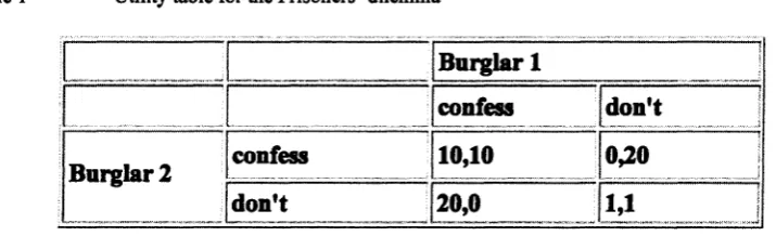
A matrix form representation, called the utility table, is used to present the

possible actions and outcomes in a game. A very popular example is the Prisoners'

Dilemma. Here, two burglars are captured and interrogated separately. They are given a

choice of either confessing or remaining silent. If both confess, they get 10 years of

prison each. If both remain silent, they get only 1 year or prison each. Finally if one

confesses while the other remains silent, the one that confesses goes free while the other

gets 20 years of prison. The results are summarized in table 1.

Table 1 Utility table for the Prisoners’ dilemma

Burglar 1

confess don't

Burglar 2 confess 10,10 0,20

don't 20,0

u____.J

The way to solve this game is to consider how burglar 1 will think: “If burglar 2

confesses, I will get 10 years if I confess, and 20 if I don’t, so it’s better to confess. But,

on the other hand, if he remains silent, I will go free if I confess or get 1 year if I remain

This means that if both prisoners act rationally, they will choose to confess.

Although this is not the optimum solution, it’s the safest, and it is what economists call

“dominant strategy equilibrium”.

The previous example does not represent the Nash equilibrium, since outcome can

be improved if players change their decisions. A Nash Equilibrium problem will be

presented in the following example.

Suppose two companies, X and Y, are producing two products. If both produce

product 1, they get a payoff of 10. If both produce product 2, they get a payoff of 5.

Finally, if both produce different products, they get no payoff. The results are

summarized in table 2.

Table 2 Companies’ utility table

Company X

Product 1 Product 2

Company Y Product 1 10,10 0,0

Product 2 0,0 5,5

In this case, the best strategy is chosen when one player chooses his move. The

other then responds using his best strategy. This is an example of a co-operative game,

and the chosen outcome is a Nash Equilibrium. It is obvious here that we have two Nash

Equilibrium points: the (product 1, product 1) point and the (product 2, product 2) point

The best overall solution will be (product 1, product 1) but the players may agree to stick

1.3 Thesis Organization

The rest of the paper is organized as follows. Section II provides a survey of the

sensor network lifetime related studies. Section III explains how the network lifetime

problem is tackled from a game theory point of view, and how this develops into

effective model that can be used to extend the lifetime of sensor networks. Section IV

then presents the simulation results along with an analysis of the results. Finally, section

CHAPTER II

REVIEW OF LITERATURE

The aim of this chapter is to give an overview of the state of the art in tackling the

energy related problems with sensor networks.

The main problem with sensor networks is limited energy availability. This is

because sensors work on batteries and stop functioning when the batteries die. Energy is

consumed when a sensor transmits data and also as it receives data. Sensor networks are

usually deployed in rough environments where it is difficult to reach the nodes for

repairing or even recharging them. It is therefore economically advantageous to

maximize the network’s lifetime. To do so, many protocols have been suggested. Some

focus on energy efficient routing while others focus directly on sensor network lifetime

optimization. On the other hand, for event detection networks, media access control

(MAC) and sleep-wake synchronization are the main issues to be considered.

2.1 Energy Efficient Studies

In [11], the authors presented five different power metrics for choosing routes in

wireless ad hoc networks. Those are: 1) Minimizing the energy consumption per packet

for all packets, which does not necessarily mean optimizing the network lifetime since

more pressure is put on certain nodes. 2) Maximizing time to network partition, which is

not very feasible when delay and throughput are a concern. 3) Minimizing variance in

node power levels, which leads to an optimization in network lifetime if the length of the

packets are carefully treated. 4) Minimizing the cost per packet for all nodes, where a

remaining energy in the nodes. A careful selection of the cost function is very crucial. 5)

Minimizing maximum node cost, which also ensures an optimization in the lifetime of

the network. The authors also introduced a MAC layer protocol which introduced large

power savings. The metrics do not necessarily have to be applied as soon as the network

starts running, instead they can be applied after the defined time threshold or energy

threshold of the network is used. The metrics introduced in this paper give an excellent

guideline to the techniques that can be used in sensor networks. However, these metrics

will optimize the network lifetime if all the nodes have the same initial energy, or if all

the nodes same similar energy levels in any given time. They do not consider the case

when the nodes do not have the same initial energies.

Later in [12], Rodoplu and Meng proposed a position-based protocol that will

guarantee the network connectivity and minimize the energy consumption of the network.

Each node is capable of transmission, reception, processing data and has a low-power

GPS (Global Positioning System) receiver. The proposed algorithm runs almost

exclusively on local information and therefore requires transmission over short distances

only. This conserves the total power required for transmission and also reduces the

interference levels. The protocol is divided into two parts. First, finding the minimum

power paths from each node to the destination by identifying its enclosure graph, and

second, finding the cost (here, defined as the total power required) of sending data from a

node to the destination along the directed path. The enclosure graph of each node defines

the maximum area for which it is power-efficient for the node to search for more

neighbours. The cost is calculated by using the Bellman-Ford algorithm where power

to work for both stationary and mobile nodes and reflects the importance of utilizing local

information.

LEACH was then introduced in [13]. This technique randomly utilizes cluster-

heads in an attempt to distribute the energy load evenly among the nodes, which in effect

extends the useful lifetime of the sensor network. To do so, three main features are

implemented. First of all, localized coordination for cluster set-up and operation is

employed. This reduces the overhead in the network, along with the transmission energy

required as opposed to global functionality. Secondly, a random choice of clusters along

with their cluster heads is used. Randomness, over a long period of time, will lead to a

uniform utilization of all the nodes in the network, and therefore an even distribution in

the energy levels of the nodes. Finally, local compression is used. This means that

computation is done on a local basis, in the clusters, reducing the amount of data

transmitted in the network. Sensors select themselves to become cluster-heads based on a

certain probability and then announce their status. Other nodes then join the cluster

according to minimum communication energy. The cluster-head node receives all the

messages for nodes that would like to be included in the cluster. Based on the number of

nodes in the cluster, the cluster-head node creates a TDMA (Time division multiple

access) schedule telling each node when it can transmit. This schedule is broadcast back

to the nodes in the cluster.

The number of clusters in the system can be pre-determined by the network

depending on different parameters. In addition to reducing energy dissipation, LEACH

successfully distributes energy-usage among the nodes in the network such that the nodes

communication and minimum-transmission energy routing (MTE) and show four to eight

times lifetime extension.

The previous methods introduce an excellent guide to the path which can be

followed to conserve energy in sensor networks. Random node assignment in LEACH

improves the network performance over the long run, but not in the short run. It shows

the importance of role rotation among nodes. An improvement to the node selection

method should be introduced to guarantee that low energy nodes will be avoided. Using

GPS and finding enclosure graphs in [12] is by its self energy consuming and expensive.

Therefore a more reliable method should be introduced. A good insight to methods that

can be used is presented in [11], and can be optimized to work for sensor network

scenarios.

2.2 Lifetime Efficient Studies

In [14], Shah and Rabaey addressed the problem of lifetime maximization by

picking the next hop nodes in a probabilistic fashion. They use the fact that optimizing

energy of a network does not necessarily mean that the lifetime of the network is

maximized. Therefore, they do not utilize the minimum energy paths. Instead, they

occasionally utilize sub-optimal paths in hope to introduce some gains. Their approach

tries to achieve an equitable degradation of the nodes’ energy. They defined a set of

“good” paths and the paths are given weights depending on some energy metric. This

paper’s significance lays in the fact that it links lifetime maximization to uniform energy

depletion. The probabilistic method also proves to work on the long run, but it is not

In [15], the authors concentrated on the problem of traffic quality and energy

efficiency in ad hoc networks. They associated a utility function with each of the

network’s nodes and develop an algorithm, ORSA, aimed at maximizing the source rate

allocation and flow control strategy given a required network lifetime. There are multiple

destination nodes, and each node has a utility function based on the route between it to

the associated destination. The aim is to maximize the sum of the utility functions. The

authors do not focus on optimizing the network’s lifetime, although their proposed

algorithm proves to improve the network’s lifetime as opposed to an earlier algorithm,

minimum transmission energy (MTE) [16]. The ORSA algorithm performs better under

the condition that the source density is less than 0.5. The idea of a personal utility

function for each node is very useful here. This means that the lifetime can be extended

based on node’s performance rather than on a probabilistic method.

The authors in [17] extended their work in [18] to include the effect of different

network topologies and the work is done on aggregating networks (i.e. where fusion of

several data streams into a single stream occurs). They assigned roles to nodes which are

composed of one or more of the following: sensing, relaying or aggregating. The role

assignment technique proves to be a powerful tool that converts the problem into a linear

one. However the computations are complicated and not all role assignments can be

solved in a similar fashion.

In [19], Dasgupta and Namjoshi presented an approximate scheme to solve the

problem of maximum lifetime data aggregation problem in sensor networks. Their goal is

not to propose a new collaborative protocol that leads to greater network lifetime. Rather,

achieve. This is an improvement to their work done in [20], where they introduced the

notion of aggregation trees which are trees that indicate how values from various sensors

are gathered, aggregated, and then transmitted to the base station. The main problem was

the complexity of the calculations for large networks. The basic operation in such

systems is the systematic collection of sensed data and eventually transmitting it to the

base station for processing. The main goal behind data aggregation is to eliminate

redundant transmissions and thus save energy. In [19], they presented two algorithms for

intelligent selection of data aggregation trees. The first one, referred to as the A-LRS

algorithm, is based on the work done in [27] by Lindsey, Raghavendra, and Sivalingam.

Here some nodes are classified as leaders, and they have the job of collecting the data,

aggregating it, and then passing it on to the next level. The second algorithm, A-R-LRS,

relies on greedy clustering of the sensors into chains, such that each sensor transmits to a

close neighbour. Using P permutations in the sensors, where P is a small constant, adds

an additional number of P*n aggregation trees. This introduced an improvement in the

lifetime of the network.

The authors in [21] focused on energy efficient routing protocols for smart badges

used in disaster situations. Their work is the same as Chang and Tassiulas in [22], except

that they added the constraint of limited bandwidth and low node energy. They

introduced metrics that balance energy consumption rates along a path in proportion to

the energy reserves of the nodes but they do not consider remaining energies of the

neighbouring nodes. Those metrics were applied on the traditional protocols and

improved the lifetime of the network by up to 60% compared to conventional minimum

lifetime. Linking node utility directly to nodes’ energy levels is an inspiring technique

which I used in my proposed protocol.

In [23], Rai and Mahapatra attempted to obtain a mathematical formulation for

the lifetime of a network. They assume that the amount of data generated by a node is

proportional to the area it covers and data generation at any individual node is a random

process. An approximate CDF is obtained that matches the simulation results. Their

mathematical result for expected lifetime and its probability distribution closely validates

the simulations results.

The authors in [24] attempted to combine concepts presented in trajectory-based

forwarding with the information provided by energy maps to determine routes in a

dynamic fashion. Data dissemination is the data communication from the monitoring

node to a set of sensing nodes that need that information. The results reveal that the

energy spent with data dissemination activity can be concentrated on nodes with high

energy reserves, whereas low-energy nodes can use their energy only to perform sensing

activity. In this work we study the problem of energy-efficient data dissemination. The

authors tiy to determine energy efficient routes based on available energy maps. They

generate trajectories that pass through regions with higher energy reserves and avoid low-

energy nodes. They then introduce a packet forwarding mechanism that eliminates the

need for neighbour table maintenance and presents a more robust behaviour in a dynamic

topology scenario, where nodes can periodically go into sleeping mode. The utilization of

energy maps for role assignment proves to be another useful method for energy

conservation. However, in my proposed algorithm, I will use energy maps in a reversed

When using Bluetooth in applications where multihop routing is required, groups

of Bluetooth piconets combine together to form a scattemet. The authors in [25] proposed

an energy-aware forwarding scheme, based on local information only, that results in an

even network resource utilization and hence an extension in the network lifetime.

Another important result is preventing critical nodes from depleting their energies. Nodes

with more energy are preferred over nodes with less energy. It has been observed that the

sensor battery life linearly declines with current consumption. Therefore, the decision of

whether to forward or not be based on the current level of the node’s battery. The

protocol succeeds in improving the network lifetime, and also in controlling the traffic

along overloaded paths.

The two main techniques used for lifetime maximization schemes are: 1) node

role assignment, through assigning more energy consuming tasks to nodes with higher

energy levels and 2) degrading energy levels at a constant rate. I will use these two points

as a guideline to my proposed protocol.

On the other hand, the main problem is that no specific criteria are presented for

the nodes to follow and base their decisions; i.e. random operation is usually

implemented. In my proposition, I will overcome this problem by introducing a cost

function that depends on each node’s status in the network. There will therefore be no

probabilistic or general approaches. Instead, a node low on resources will be avoided and

CHAPTER III

DESIGN AND METHODOLOGY

In this chapter, we present the development of the life-extending protocol through

detailed game theory analysis. By the end of this chapter, we will gain an understanding

of the basics upon which the protocol runs.

3.1 Introduction

Network lifetime is defined as the number of packet transmissions a network can

perform before one node, or a percentage of the nodes, dies. Node lifetime is defined as

the number of packet transmissions the node can perform before it runs out of energy and

can be estimated using the following equation:

L t : Node lifetime,

e i : Node’s remaining energy,

&txi : Energy required per transmission.

Since sensor networks usually operate in rough conditions, such as battlefields or

under the ocean, repairing or recharging nodes becomes a very difficult task. The only

feasible solution is usually to replace the network. This means that as soon as the network

lifetime expires, new nodes are thrown into the area to form a new network and the old

network is disregarded. Therefore, it is economically and practically essential to

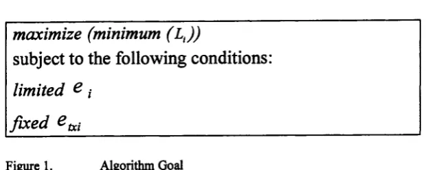
The main goal is to achieve the following:

maximize (minimum ( L j )

subject to the following conditions:

limited e ,•

fix ed e M_________________________________________

Figure 1. Algorithm Goal

According to Nash, the best result is achieved if each player (node) does what is

best for him self and the entire group (the network). It is therefore our goal to come up

with a protocol where all the nodes co-operate in order to maximize both their own

lifetime while considering the lifetimes of the other nodes, i.e. the network lifetime.

The development of the model will be presented in the following section.

3.2 Model Development

From formula (1), it is obvious that a node’s lifetime is directly proportional to

the amount of energy it carries and inversely proportional to the energy it spends per

transmission:

L t a e

L t a 1 i e ui

It is therefore logical to use nodes with higher energies and avoid nodes which use

more energy per transmission in order to increase the network lifetime.

Now let’s assume that we have to choose between two neighbours to relay the

data. One of them has a much higher energy reserve but will consume much more energy

and die. In terms of energy conservation, it is better for the whole network, and for the

first node, to use the second node. But in terms of network lifetime, it is better to use the

first node since this will leave us with no dead nodes and the network can continue to

function. This draws our attention to another important point. The nodes’ energies should

be degraded at a constant rate in order for all the nodes to enjoy a higher network

lifetime. Therefore, the nodes should co-operate together to maximize their utility. This

example shows the difference between focusing on energy conservation and life time

extension.

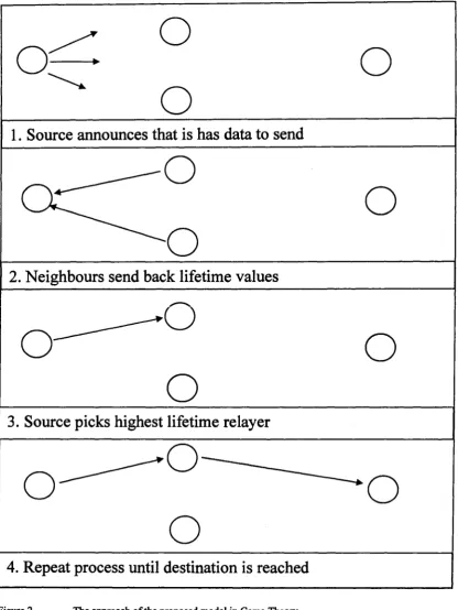
Therefore, tackling the situation from a game theoretic approach can be visualized

as follows. Each node calculates its average expected lifetime as in formula (1). When a

source announces that it wants to send some data, all the neighbours send their lifetime

values to the source and the source picks the node with the highest lifetime value. The

o

°^r

o

o

1. Source announces that is has data to send

o

2. Neighbours send back lifetime values

O

""'*0

_o

o

3. Source picks highest lifetime relayer

-o

o

4. Repeat process until destination is reached

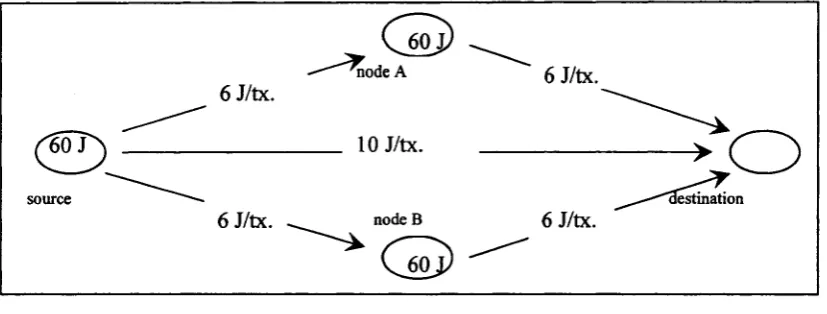
3.3 A Numerical Example

We will analyze a simple 4-node network in a Game Theoretic approach to

illustrate the validity of the model. Let us assume that we have a source attempting to

send data to the destination, with two possible relayers in between. There are four

possible scenarios. The first one is the basic operation, where both possible relayers act

selfishly and decide not to co-operate. The second and third scenarios occur when only

one of the nodes co-operates and finally in the final scenario, both nodes co-operate. We

assume that all nodes have an initial energy of 60 J, and the energy required per

transmission is proportional to the distance between the nodes.

node A _{6 J/tX.}

6 J/tx.

10 J/tx. 60 J

lestination source

6 J/tx. 6 J/tx. node B

The 4-node network Figure 3.

o

node A

o--->o

source destination

nodeB

As we can see in Figure 4, with an initial energy of 60 J and a required 10

J/transmission, source is able to perform 60/10=6 transmissions. Therefore the lifetime of

the network in this case is 6.

node A

destination source

nodeB

Figure 5. Node A co-operates.

In this case, node A decides to relay data. Although node A now spends energy, it

is better off because the lifetime of the network becomes 60/6= 10. We also realize that

node B has benefited the extended lifetime without spending any energy.

node A

destination source

nodeB

CD

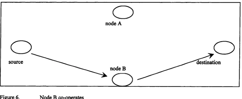
Figure 6. Node B co-operates

In this case, node B decided to relay. The situation is inversed. Here node B

spends energy to extend the network lifetime to 10 transmissions, while node A benefits

node A

o.

destination source

node B

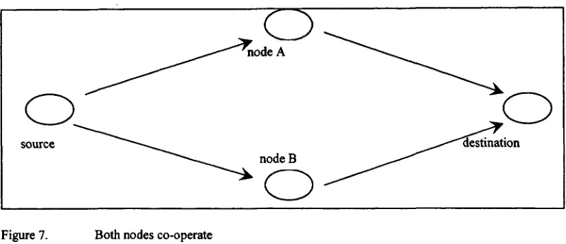
Both nodes co-operate Figure 7.

Finally, both nodes decide to co-operate. Half the data is relayed through node A

while the other half is relayed through node B. Each of them achieves 5 transmissions,

and therefore the overall lifetime is still 10. The advantage here is that both nodes co­

operated and shared the effort in extending the lifetime.

Now, we will analyze all four scenarios in a Game theoretic approach.

Scenario 1: No co-operation

This is the basic operation of the network, and all others will be compared to this

one. Here we have a network lifetime of 6 transmissions. Nodes A and B do not spend

any energy and the source depletes all its energy in the transmissions.

Now defining the utility function as lifetime extended per unit energy spent as

opposed to the basic operation, we obtain the following.

Scenario 2: Node A co-operates

All data is relayed through node A. Lifetime is extended from 6 to 10

transmissions with an expenditure of 60 J from both node A and the source. Node B does

Lifetime: 10

Lifetime extension: 10-6=4

u(S): 4/60=0.0667

u(A): 4/60=0.0667

u(B): 4 /0 = o o

Scenario 3: Node B co-operates

All data is relayed through node B. Lifetime is extended from 6 to 10

transmissions with an expenditure of 60 J from both node B and the source. Node A does

not spend any energy.

Lifetime: 10

Lifetime extension: 10-6=4

u(S): 4/60=0.0667

u(A): 4 /0 = o o

u(B): 4/60=0.0667

Scenario 4: Both nodes co-operate

Half the data is relayed through node A and the other half is relayed through node

B. Lifetime is 10 transmissions. Nodes A and B spend 30 J each while the source depletes

all its 60 J.

Lifetime: 10

Lifetime extension: 10-6=4

u(S): 4/60=0.0667

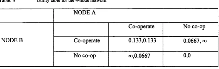
And representing the previous results in a utility table, we get:

Table. 3 Utility table for the 4-node network

NODE A

NODEB

Co-operate No co-op

Co-operate 0.133,0.133 0.0667, oo

No co-op oo,0.0667 0,0

As shown, (co-operate, co-operate) represents the Nash equilibrium point, since

no node can improve his performance without degrading the other node’s performance.

Therefore, co-operation of all nodes in the network, works out to be the best.

3.4 Formulation

3.4.1 The governing formula

We now need a cost function that will reflect the previous behavior. The function

should govern the behavior of the data transmissions and have the following properties:

1) Encourage use of nodes with more energy reserves

2) Discourage high power transmission links

3) Function with different node energy scenarios, whether the nodes have same

initial energies or variable energy values

4) Scalable, which means that the protocol should function well with increasing

network size

5) Degrades the energy values of the nodes at a uniform rate

exj + 1 / pii

p ij: energy of transmission,

c ij: cost of transmission, and

exj: difference between neighbour node’s energy and average energy of nodes:

6 X j = € j — 6 average ( 3 )

The significance of introducing exj is to compare a node’s energy with its

neighbours’ energy values. This will achieve uniform energy degradation throughout the

network.

The decision to be made is to choose a relayer from the neighbouring nodes. In

doing so, the source will consider two criteria: (i) difference between the remaining

energy in the nodes and their neighbours and (ii) transmission energy, used in sending a

packet from one node to the other. By introducing the first criterion, we intend to keep

relaying nodes alive as long as possible by using nodes whose energy level is relatively

higher than others. The cost function encourages the use of a relayer that is better in

terms of remaining energy as opposed to neighbours at each packet transfer. This will

alternate use of relaying nodes and allow them to improve network lifetime. The second

criterion is to pick a relaying node that uses minimum transmit power.

3.4.2 Algorithms

We provide two algorithms to implement our approach. One is based on global

knowledge, and the other is based on local knowledge. In global knowledge, every node

knows the expected lifetime of all other nodes. We assume that that information is

node to other nodes is complex and requires additional protocols, which can consume

large network resources, such as bandwidth and energy. But that approach will provide us

with better understanding on how the algorithms behave.

The second approach is based on local knowledge. How the information is

disseminated is not an issue in the design here. But disseminating local information to

neighbours is a much easier and manageable task than disseminating all information to all

the network nodes. Information can travel through the network simply by nodes listening

to their neighbours, without increasing the network overhead. We now discuss those two

approaches.

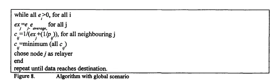
The Global Knowledge based approach is given by Figure 8. When node / has a

data packet to send out, it calculates the cost of sending that packet to the next hop node j,

c . Node j then picks the next hop, and so on.

w hile all e >0, for all i

t 9

ex~e e for all j

j j - a v e ra g e,

c = \l(e x + {\lp .)), for all neighbouring j

c = m inim um (all c )

'] <J

chose n ode j as relayer end

repeat until d a ta reaches destination.

Figure 8. Algorithm with global scenario

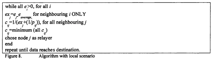
The Local Knowledge based approach is given by Figure 9. It is similar to global

knowledge approach, but in the local approach, only the information obtained by

while all e >0, for all i i

ex=e e for neighbouring i ONLY

j f average,

c=\l(ex+(\lp^)), for all neighbouringy

c =minimum (all c )

ij 'J

chose node j as relayer end

repeat until data reaches destination.____________________________________________

Figure 8. Algorithm with local scenario

We would like to emphasize one more time that the local knowledge based

approach is more feasible than global knowledge based approach. When we consider that

the nodes only forward packets to next hop, which is a neighbouring node, the local

knowledge based approach should not deviate much from the global approach but

operates with much less overhead [28].

The energy model used to calculatepy is based on the work done in [13] where:

■Ee/ec=50nJ/bit is the energy required to run a transmitter or receiver circuit,

Eamp= 100pJ/bit/mA2 for the transmitter amplifier, receive and transmit powers

become functions of k bits:

3.5 Minimum Hop and Minimum Energy Routing

The proposed algorithm will be compared to the two most common routing

protocols; the minimum hop (MH) and minimum energy (ME) routing protocols. In order

to obtain fair results in the long run, an estimation technique is introduced. The results are

an average of at least 1000 simulations. The approach used to simulate both algorithms is

explained in the following two subsections.

rx,—Eelec*k (4)

3.5.1 Minimum Hod Routine Protocol

The minimum hop protocol will be simulated using an estimation formula that

will implement the best case scenario. The data packet will be assumed to travel in a

straight line, therefore when a node has data to send, the number of hops required to

reach the sink is the distance between the source and the sink divided by the node range

[26]

h = d(source, sin k) ₍₆₎

h: Number o f hops

d ( ij) : D istance between nodes i and j

r: N ode range

[jtJ: Operation rounds the elem ent to the nearest integer greater than or equal

to it

sink 1

sink

source

Figure 10. Minimum hop estimation

Procedure:

1. find distance between source and all sinks: d(s,l) and d(s,2)

2. choose sink of minimum distance: sink 1

3.5.2 Minimum Energy Routing Protocol

The minimum energy protocol will be estimated using a more complicated

technique. Using the facts that the node distribution is random and the results are

repeated and averaged over at least 1000 simulations, we assume the node distribution to

be uniform in the long run. Minimum energy protocol searches for the route with

intermediate hops where the total distance traveled is smallest per hop. This is because

the received power at on node is proportional to dfl where d is the distance between the

source and the sink and B is the path loss exponent, which in my simulations is assumed

to be 2.

According to the previous assumptions, we work on a uniformly aligned network

as shown below.

o o M

o o o o

o

o o o o o o o

o o o o o o o o o

Figure 11. Minimum energy estimation

Procedure:

1. find distance between source and sink

2. find number of hops according to previous assumptions

The distance between each two nodes, horizontally or vertically, is Ju where u is

the uniform node density. And the diagonal distance is V“2 + «2 . The transmission

powers are then calculated accordingly.

In this chapter, the basics of the protocol were explained. An example was used to

verify the validity of the method in terms of game theory. Finally, the technique used to

estimate the performance of the networks using the minimum hop routing and the

minimum energy routing protocols is introduced. In the following chapter, the protocol is

put into practice and its performance is tested and analyzed. Modifications will be

CHAPTER IV

ANALYSIS OF RESULTS

4.1 The Sample Model

This model was introduced in the first stages of the model development to test the

cost function on a small scale before extending the work. Figure 12 presents the

simulation topology. In that topology, there are 11 nodes, including source and

destination, and 4 tiers (i.e., 4 hops). The selection of a relayer will be within the tier. For

example, the source has to select one of the following nodes: 2, 3 or 4 to be its relaying

node. The selected node (2, 3, or 4) then has to select a relayer between node 5 and node

6, and so on.

The simulations were performed using MATLAB. We ran several different

scenarios with this topology. First, node energies are distributed randomly, to mimic the

scenario where utilization of the nodes is not uniform. Then we assume that the initial

energies are equal.

200 150 100 50 sou ce

c

o

o

o

o

o

o

o

o

o

o

In the simulations, we compared the proposed “global knowledge based”

approach, the proposed “local knowledge based” approach, “minimum energy route”,

“maximum available energy approach” and an “arbitrary (i.e., random)” relayer selection

approach. In all approaches, the transmitting node consumes energy based on distance

between the nodes. It is also assumed that each node consumes fixed amount of energy

when it receives a packet regardless of the separation.

Figure 13 shows the final energy levels of the nodes after the simulation ends with

each approach. In that scenario the initial node energies are distributed randomly.

Simulation ends when any of the nodes dissipates all of its energy. In that figure,

proposed global and proposed local leave nodes with energies that are more uniformly

distributed. Although some of the node energies are more in other approaches, since

some nodes depleted their batteries earlier, the network lifetime is relatively short

compared to the proposed approaches. The proposed approach is better, since lower final

energies in the nodes indicate that the nodes were utilized to their maximum capacity to

extend the lifetime of the network. A node with energy when the network stop

Different initial energy nodes

3

- • - g l o b a l

lo ca l

■ m in im u m e n e r g y

>K m ax . a v a ila b le e n e r g y

e a rb itra ry

Figure 13 Final energies o f nodes in scenario where nodes have different initial energies

Figure 14 shows the final energy levels of the nodes after the simulation

ends. In that simulation, the nodes’ initial energies are equal. That Figure shows

that the proposed algorithm’s approaches leaves nodes with relatively uniformly

distributed energies, in other words, network nodes dissipates their energies more

evenly. That allows network to survive longer.

Same Initial energy nodes

1 2 0

1 0 0 - global

local

minimum energy

arbitrary

node

Tables 4 and 5 present comparisons of the number of packets sent in each

approach. As the table reveals, the proposed approaches have the longest lifetimes. It is

interesting to note that the proposed local algorithm is almost 25% better than the

proposed global algorithm and nearly 50% better than others. That can be explained by

each node’s lifetime is degraded as opposed to its neighbours only.

Table 4. Case where nodes have different initial energies

Protocol Proposed (global) Max. available energy route Minimum energy route Arbitrary Proposed (local)

Packets sent

(lifetime)

68 60 50 53 85

Table 5. Case where nodes have same initial energies

Protocol Proposed

(global)

Max. available

energy

Minimum

energy route

Arbitrary Proposed

(local)

Packets sent

(lifetime)

77 67 64 95

Here we presented a trial model that improves lifetime of a sensor network by

allowing nodes to alternate during packet forwarding. In that algorithm, nodes select a

relaying node that has the longest expected life time. Our simulation results show that

this algorithm (approach) maximizes lifetime compared to other approaches, namely

“minimum energy routing”, “maximum available energy routing”, and “random routing”

by almost 50% on average.

As the primary results seem promising, the next step becomes extending the

4.2 The Network Model and Results

A uniform node density of 4000 m2/node will be assumed throughout the

simulations. Nodes will be assumed stationary, and will expend energy upon transmitting

and receiving energy according to the energy model from [13]. Fifty percent of the nodes

will be assumed possible sources and ten percent as sinks. All nodes will be randomly

allocated; nodes within the simulation area and sinks around the network boarder as

shown in Figure 15. Overhead energy is ignored, as this is a small percentage compared

to the overall spent energy [6],

X X

r X _ X X

* • X

800

m

m

X

X

100

X

100 800 800

Figure IS. A randomly allocated network

The MATLAB code written will be able to perform a variety of functions, and

collect a vast amount of data by implementing the techniques used in Network Simulator,

NS2. These include overhead, next hop, number of hops, number of data packets sent and

network lifetime.

The code will implement the local scenario, where each node uses only its

the next node until the destination is reached. The results are presented in the next

section. As shown in Figure 16, a source will send out a request, and its neighbours will

respond by sending back their energy level values. Based on the energy level values, and

the distance between the source and the neighbours, calculated by measuring the power

loss, the source will calculate the cost to each neighbour. The source will then pick the

cheapest neighbour to send the data packet to and the process is repeated until the

destination is reached.

nw ' r

««■*

v i Q

-1. S ource requests neighbors' inform ation

0.0

2. N eighbors send back th e ir energy levels

X....’h

■ - T © ,

oo

3. Source calculates cost and sends data to cheapest node

. m w - f

■;

4. P ro ce ss re p eated u n til sink is in rcnch

Figure 16. Algorithm steps

The protocol is run on different size networks using MATLAB. The maximum

number of nodes simulated was 2800, but the number can be extended. Two different

cases where studied. The first of which lifetime is defined as the time when the first node

dies, and the second is when 25 percent of the nodes die. Snapshots of a 200 nodes

network where taken to represent the network condition when one node dies, and then

when 25 percent of the nodes die. These are presented in Figure 17. This shows the

energy, and the dead nodes are marked with Xs. Destinations are randomly distributed

around the edge of the network and represented as red stars.

• n • • I

* j

•

* - ? • • * •«

x

*

$ S '

i

• s .

f*

x A •• ' • • . f* X A •*

/V

JC

'* I*' i* >

?

V

.*

&

*

>

*

%

• *

£ • •* 2 1 '*

I*

x«£*x

4 % ? , • • • * . , . « . s % x V

% •

• J

•

9

X X - X X

X x x

X

Figure 17. Network snapshots when a) one node dies, b) 25% o f nodes dies

Since the protocol is allowed to run without any sense of direction, i.e. it is

entirely based on the cost function, sometimes unnecessary paths will be taken and the

packet will end up traveling a much longer distance. This case is represented in Figure 18

along with another scenario where the packet takes an efficient path.

JL

• •

» •

M l

• •

•

• •

M.

Figure 18.

150 200 290 300 350 w 400 0 90 100

Both a)Inefficient path and b) efficient path

200 290 300

When simulated, the minimum hop protocol is assumed to perform at its best

Nhops = d,to sink (6)

threshold

Where

[J

equal to it.

The number of hops required for the proposed algorithm reflects the latency. It is

plotted, as shown in Figure 19, as opposed to the ME and MH protocols, which are

obtained as explained in the previous chapter.

Due to the absolute dependence of the proposed cost function on the transmission

energy and the nodes’ energy levels, the number of hops increases with the number of

nodes, since unnecessary paths become more common as networks grow in size.

22

o 100 200 300 400 500

N odes

The number of packets sent, which represent the lifetime, is next plotted for both

lifetime definitions in Figure 20. The figure demonstrates the advantage of defining the

lifetime as when 25% of the nodes die over when lifetime is defined as one node dead.

This is because the probability of one node dieing is independent of the network size.

Therefore, better network utilization is achieved when terminating the network as soon as

25% of the nodes die.

350

300

jjs 250

U-200 _{25 % DEAD}

LU

%

100 _{1 NODE DEAD}

50

50 100 150 200

NODES

250 300 350 4 00

Figure 20 Packets sent; for different lifetime definitions

As a means of comparison, the energy per packet metric is introduced. This

metric measures the utility of the network. It will be denoted as EP for short, and

measured in J/packet. It is used as a means of comparing the performance of the

introduced protocol to both the MH and ME protocols. Its value is measured by dividing

MH

0.8

CJ

0.6

PR O PO SED

CD Q£

Z 0.4

■O

ME

0.2

200 600 800 1000

NODES

Figure 2 1 EP vs. nodes for MH, ME and proposed

As observed from Figure 21, the proposed protocol performs much better than the

MH up to around 700 nodes and better than the ME up to around 180 nodes. This is

mainly due to the higher rate of increase in hop count for the proposed protocol as

opposed to the other two. This triggers the need for an optimization of the cost function.

The modification we introduce will be considering the distance of the node from the

closest sink. This should help direct the data packet into a straight line towards the sink,

thus reducing the number of hops, and hence the EP value. The cost function will be

modified as follows:

=--- — ---v Kd * d( j,closest _destination)

«*0') + —tttt (7)

P i h j )

kd is a constant that balances the weight of both terms of the modified cost

function. The previous results will be re-plotted to test the modified cost function, and are

25 r

20

P R O P O S E D 15

1 0

MODIFIED ME

5

MH

O.

O 100 200 300 400 500

NODES

Figure 22 Hops vs. nodes; MH, ME, proposed and modified version

Figure 22 shows how the modified protocol introduces a great improvement in the

network’s latency over the original proposed protocol. Also, the number of hops for the

proposed algorithm is slightly larger than that of the MH and ME. The results will be

extended to 2800 nodes to check the performance of the modified protocol at such

network size, as shown in Figure 23.

1*1

10

C O

Next, we will show the impact of the modification on the EP value.

x 10 1.2 Id o . MH 0.8 az

u j 0.6

s -o or 0.4 PRO POSED U J z U J ME MODIFIED 0.2

200 400 600 800 1000

NODES

Figure 24 EP vs. nodes; M H, M E, proposed and modified version

Once again, it is obvious how the modified cost function improves the

performance of the network and extends its lifetime.

It is important to bear in mind that the protocols do not consider the overhead

energy, and also the GPS energy needed in the modified case is ignored.

In this chapter, we proved the validity of the proposed protocol by applying it to a

small sample network. Since the results seemed promising, a network model was created

and the protocol was allowed to run on bigger networks. The proposed protocol works

fine in terms of lifetime extension, but caused an increase in latency as the network got

bigger and bigger. Optimization of die protocol was then suggested, and the optimized

protocol works a lot better in terms of lifetime and latency. A more comprehensive

CHAPTER V

CONCLUSIONS AND FUTURE WORK

5.1 Conclusions

The game theory proved to be a strong and effective tool for optimizing the

performance of wireless networks. In this thesis, the game theory was used as a guideline

by which the nodes in a network will base their decisions to extend the overall lifetime.

Nodes cooperated and exchanged information with their neighbours in order to achieve

uniform energy degradation across the network. This, in effect, resulted in lifetime

extension.

The network, using the proposed algorithm, depleted its energy in an inside-out

fashion. This means that the nodes closer to the center of the network tend to loose their

energy faster than the nodes closer to the border. This is because border nodes are usually

closer to sinks, and therefore will be used much less.

The introduced cost function was a major key in the success of the protocol. It

eliminated the randomness, which was usually applied in previous research, and

introduced guidelines to relayer selection.

The proposed protocol is advantageous over both the minimum hop routing

protocol and the minimum energy routing protocol in terms of energy per packet, i.e.

lifetime, up to 700 nodes for the first case and 180 nodes for the latter case. It should be

taken into consideration that the ME and MH protocols were simulated using estimation

techniques that give advantage to their results.

The modified proposed protocol introduced a huge improvement in terms of both

enhanced nodes. This means an increase in the network cost which might not be feasible

in some cases.

5.2 Future Work

The results obtained using MATLAB confidently indicate an improvement in

performance over conventional communication protocols. Yet, it still remains necessary

to verify the results using network simulator tool NS and also to include the overhead

energy, which was ignored in MATLAB.

Also, a number of factors used in the simulation can be examined and optimized.

These include the metric, the node density, and different lifetime definitions.

I expect the protocol performance to resemble that of the minimum hop protocol

as the metric is bigger, i.e. more weight is given to the distance between the node and

the sink. Node density and source density, which was assumed to be 50% in my

simulations, should also have an impact on the protocol performance. I predict that a

higher node density should increase the latency of the network when using the proposed

protocol and possibly also increase the lifetime. The value of the node density should be

optimized according to the desired specifications.

Finally, different lifetime definitions will affect the utilization of the nodes.

Various values should be examined to study the effect on node utilization and success

rate. In my thesis, I studied the network for two lifetime definitions only: when one node

dies and when 25 % of the nodes die. A larger definition means that the protocol will

continue to run until more nodes die. This might cause some nodes to be isolated and

therefore unable to send out data packets. This will increase the failure rate. Therefore, an