Localization for Mixed Near-Field and Far-Field Sources
by Interlaced Nested Array
Sheng Liu*, Jing Zhao, Ziqing Yuan, Ren Zhou, Min Xiao, and Chunyan Lu
Abstract—In this paper, a localization algorithm for mixed near-field and far-field sources by an interlaced nested array is proposed. The fourth-order cumulants (FOCs) of the received data are used to construct a FOC matrix, by which the angles of all signals can be estimated. Then, an effective method is driven to separate the directions of arrival (DOAs) of near-field and far-field sources without extreme value search. The ranges of the near-field sources can be estimated by one-dimensional (1D) search. Compared with existing nested array-based algorithms, the proposed algorithm can distinguish more sources and has higher estimation accuracy. Some simulation results are shown to certify the superiority of proposed algorithm.
1. INTRODUCTION
Localization of space signals is a key technology in radar, mobile communication, etc. Far-field signal wave is seen as a plane, so we localize the far-field source only by estimating its direction of arrival (DOA). There are many classic DOA estimation algorithms for far-field sources such as MUSIC algorithms [1, 2], ESPRIT [3], and propagate method (PM) [4].
For a near-field signal, the hypothesis of plane wave does not hold, and it propagates as spherical wave. The estimations of DOA and range are needed to locate the near-field signals. Two-dimensional (2D) MUSIC algorithm [5] gets estimations of the DOA and range by 2D searching, but the computational complexity of this algorithm is too high. In order to avoid 2D search, many methods [6– 8] first estimate DOA separately. Then, by using the estimated DOA, the range can be estimated by several times of one-dimensional (1D) search. A generalized ESPRIT is proposed for the DOA estimation of near-field source via symmetric array in [6]. In [7], Jiang et al. estimate the DOAs of all far-field and near-field signals by separating the angle information from the steering vector. However, for methods [6, 7], the angles search procedure involves repetitive computations of determinant, which is also a high complexity process. In [8], He et al. use partial elements of a covariance matrix to construct a new cross-covariance matrix which is only related to the angle information. However, in order to separate the angle information, both the algorithms [7, 8] can cause aperture loss, which reduces the accuracy of locating and cuts down the number of identifiable signals to some extent.
In order to remedy the aperture loss, some FOC-based algorithms [9–12] have been proposed to increase the virtual sensors. In [10, 11], Zheng et al. exploit second order statistic (SOS) to estimate DOAs of far-field sources, and a FOC matrix is exploited to estimate the DOAs of near-field sources after removing the information of far-field sources. In [12], a FOC-based PM algorithm is proposed for the localization of near-field sources. In fact, besides FOC, using sparse array is also an effective way to reduce aperture loss. Recently, many efficient sparse array architectures such as co-prime array [13] and nested array [14, 15] have been proposed, and many localization algorithms [16–18] have been proposed based on these sparse arrays. In [16], a localization algorithm for near-field sources based
Received 25 April 2019, Accepted 5 June 2019, Scheduled 26 June 2019 * Corresponding author: Sheng Liu ([email protected]).
on the symmetric co-prime array is proposed. The symmetric nested array and symmetric interlaced nested array are proposed for the localization of mixed near-field and far-field sources in [17] and [18], respectively.
Besides the algorithms mentioned above, many other algorithms including oblique projection method [19] and spatial differencing method [20] are also proposed for the localization of near-field and far-field sources and show advantages in reducing computational complexity or improving the precision of localization. In [21], an algorithm based on rank reduction is presented for the localization of near-field and far-near-field non-circular sources. For this algorithm, a non-circular property of source is utilized to improve the performance of the parameter estimation.
In this paper, a localization algorithm for mixed near-field and far-field sources by an improved interlaced nested array is proposed. The FOCs of the received data from an improved interlaced nested array are used to construct a FOC matrix. The angles of all signals can be estimated by dealing with the FOC matrix. Then, a fast method is driven to separate the DOAs of near-field and far-field sources. Compared with the nested array-based algorithms [17, 18], the proposed algorithm shows three advantages: (1) the proposed algorithm can distinguish more signals than [17, 18]; (2) the proposed algorithm shows more estimation accuracy than [17, 18]; (3) the proposed angle separation method has lower complexity than [17, 18].
Notation: [•]T, [•]∗, [•]H, and E[•] stand for transpose, conjugate, conjugate transpose, and statistical expectation, respectively. c[i:j] denotes the vector consists of the ith component to thejth component of vectorc. Jrepresents a matrix with 1 on the back diagonal and 0 on the other positions.
2. RECEIVED MODEL
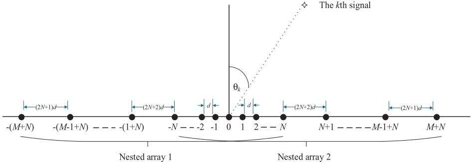
Consider an interlaced nested array consisting of two nested arrays [15] shown in Fig. 1. The po-sitions of the sensors are {−[M(2N + 2) + N −1],−[(M − 1)(2N + 2) + N],· · ·,−[(2N + 2) +
N], −N,−N + 1,· · ·,1,0,1,· · ·, N −1, N, (2N + 2) + N,· · · ,(M − 1)(2N + 2) + N, M(2N + 2) + N − 1}d, where d is the unit element spacing with (d = λ4). Suppose that K sig-nals impinge on the array. Denote the received data vector x ∈ C(2M+2N+1)×1 as x(t) = [x−(M+N)(t), x−(M+N−1)(t),· · · , x−(N+1)(t), x−N(t), x−(N−1)(t),· · · , x−1(t), x0(t), x1(t),· · · , xN−1(t), xN(t), xN+1(t),· · · , xM+N−1(t), xM+N(t)]T ∈C2M+2N+1 and
xi(t) = K
k=1
sk(t)ej(μkli+ϕkl
2
i)+ni(t) (1)
where μk = −2πdλsinθk, ϕk = π d
2
λrkcos 2θ
k, θk is the DOA of the kth signal, li the distance between
the ith sensor to the reference sensor, and rk the distance between the kth signal to the array. When
Nested array 1 Nested array 2
The kth signal
d (2N+2)d
(2N+1)d d (2N+2)d (2N+1)d
-(M+N) -(M-1+N) -(1+N) -N -2 -1 0 1 2 N N+1 M-1+N M+N
k
θ
sk(t) is far-field signal, rk = +∞, thus ϕk = 0. When sk(t) is near-field signal, we suppose that
0.62(D3/λ)1/2 < rk<2D2/λ.
Letθ= [θ1, θ2,· · ·, θK] and r= [r1, r2,· · · , rK], then x(t) can be expressed as
x(t) =A(θ,r)s(t) +n(t) (2) whereA(θ,r) = [a(θ1, r1),a(θ2, r2),· · · ,a(θK, rK)] is manifold matrix, anda(θk, rk) can be expressed
as
a(θk, rk) =
⎡ ⎢ ⎢ ⎢ ⎢ ⎢ ⎢ ⎢ ⎢ ⎢ ⎢ ⎢ ⎢ ⎢ ⎢ ⎢ ⎢ ⎢ ⎢ ⎢ ⎢ ⎢ ⎢ ⎢ ⎣
ej[−μk[M(2N+2)+N−1]+ϕk[M(2N+2)+N−1]2] ..
.
ej[−μk[(2N+2)+N]+ϕk[(2N+2)+N]2]
ej[−μkN+ϕkN2] .. . 1 .. .
ej[μkN+ϕkN2]
ej[μk[(2N+2)+N]+ϕk[(2N+2)+N]2] ..
.
ej[μk[M(2N+2)+N−1]+ϕk[M(2N+2)+N−1]2] ⎤ ⎥ ⎥ ⎥ ⎥ ⎥ ⎥ ⎥ ⎥ ⎥ ⎥ ⎥ ⎥ ⎥ ⎥ ⎥ ⎥ ⎥ ⎥ ⎥ ⎥ ⎥ ⎥ ⎥ ⎦ (3)
3. DOA ESTIMATION OF ALL SIGNALS
We first construct a FOC vector c1 ∈C(2N+1)(M+1)×1 with
c1(l) = cum xN+t(t), x∗N+1−l(t), x∗−(N+t)(t), x−(N+1−l)(t)
(4)
wherel=k+t(2N+ 1),1≤k≤2N + 1,0≤t≤M. Then, we denote a FOC vector c2 ∈C(M−1)×1 with
c2(l) = cum xN+M(t), x∗N+M−l(t), x∗−(N+M)(t), x−(N+M−l)(t)
(5)
wherel= 1,2,· · · , M−1.
Denote two vectors e2N+2 = [0, 0,· · ·,1]T ∈C(2N+2)×1 and 1M−1 = [1,1,· · · ,1]T ∈C(M−1)×1, which can be used to construct three FOC vectors c3,c4 and c5 as
c3 = c2⊗e2N+2+
1M−1⊗
I2N+1 0
c1[1 : (M−1)(2N + 1)] (6)
c4 =
c3
c1[(M−1)(2N + 1) + 1 : (M + 1)(2N + 1)]
(7)
c5 = c4[2 : (2N+ 2)(M + 1)−2] (8)
Utilizing c5, we can construct a vector c∈C[2(2N+2)(M+1)−5]×1 as
c=
Jc∗5 c4
(9)
Using the vector c, we can construct a FOC matrix R∈C[(2N+2)(M+1)−2]×[(2N+2)(M+1)−2] by
Because the FOC of Gauss noise is equal to 0, after denotingqx= cum{sk, s∗k, sk, s∗k}, we can get
that
R=BCsBH (11)
whereCs= diag{q1, q2,· · · , qK} and B(θ,r) = [b(θ1, r1),b(θ2, r2),· · ·,b(θK, rK)] with
b(θk, rk) =
⎛ ⎜ ⎜ ⎜ ⎜ ⎝
1
ej2μk .. .
ej2μk[(M+1)(2N+2)−2] ⎞ ⎟ ⎟ ⎟ ⎟
⎠ (12)
Performing eigenvalue decomposition (EVD) ofR, we can estimate the DOAs of all far-field and far-field signals by MUSIC [1].
4. CLASSIFICATION OF SOURCE
Construct an SOS covariance matrix
Rx =Ex(t)xH(t)=A(θ,r)RsAH(θ,r) +n(t) (13) Performing EVD of Rx, we can get the noise subspace Un as [1], then denote v(θ, r) =
aH(θ, r)U
nUHna(θ, r).
It is easy to know that if θk is the DOA of a far-field signal, we have |v(θk,+∞)| = 0 and
|v(θk, r)| = 0 for any r >0.
On the other hand, ifθkis the DOA of a near-field signal, we havev(θk,+∞)= 0 andv(θk, rk) = 0.
We can also find that|v(θk, r)|increases with r changing from rk to max{r}.
According to these, we can distinguish the near-field signals and far-field signals by
v(θk,+∞)< v(θk,max(r)), θk is the near-field angle v(θk,+∞)> v(θk,max(r)), θk is the far-field angle
(14)
where max{r}= 2D2/λ.
Remark: In [17, 18], the authors use the estimated ˆθk to search the minimum value of aH(ˆθk, r)UnUHna(ˆθk, r). So, it needs to take K times global searching to distinguish the near-field
signals and far-field signals. For the proposed algorithm, we only need compute 2K values. So the computational complexity will be reduced.
5. ESTIMATION OF RANGE FOR NEAR-FIELD SIGNALS
Using noise subspaceUn, we can get the function
fMUSICk (r) =
1
aH θˆk, rUnUH
na θˆk, r
(15)
Searching the maximum offMUSICk (r), we can get the ranges for near-field signals as [16, 17].
6. SIMULATION
comparison, we use the same method to search range. The root-mean-square errors (RMSEs) of DOA estimation and range estimation are given as
RMSE =
1
KJ J
j=1
K
k=1 ˆ
θkj−θk
2
(16)
and
RMSE =
1
KJ J
j=1
K
k=1
(ˆrkj−rk)2 (17)
whereJ = 200, and ˆθkjand ˆrkjare the estimations ofθkandrkin thejth Monte Carlo trial, respectively.
The comparisons of RMSE for three algorithms are given in the case that the pairing is accurate.
6.1. Experiment 1
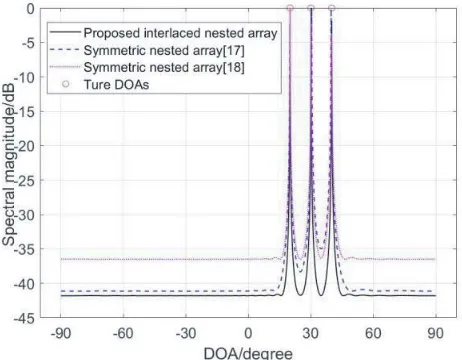
Firstly, we compare the space spectra of three methods for all sources. Suppose that SNR is 5 dB and that the number of snapshots is 500. Consider two near-field signals s1, s2 with θ1 = 20◦, r1 = 40λ,
θ2= 30◦,r2 = 45λand a far-field sources3 withθ3= 40◦. Fig. 2 shows the space spectra of 3 methods for three signals with 10◦ interval. Then, we change the DOAs of three sources intoθ1= 25◦,θ2= 30◦, and θ3= 35◦. Fig. 3 shows the space spectra of 3 methods for three signals with 5◦ interval. From the two figures, we can see clearly that the algorithm based on the proposed interlaced nested array shows higher angular resolution.
Figure 2. Space spectra of three methods for three sources with 10◦ interval.
6.2. Experiment 2
Figure 3. Space spectra of three methods for three sources with 5◦ interval.
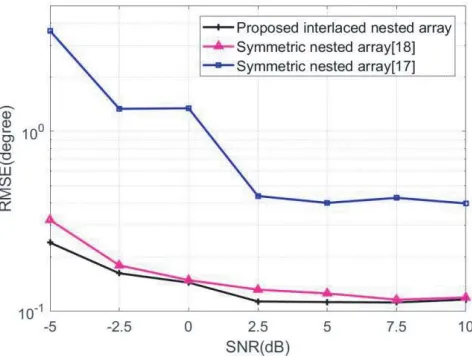
Figure 4. RMSEs of near-field angles versus SNR.
Figure 6. RMSEs of ranges of near-field signals versus SNR.
Figure 7. RMSEs of near-field angles versus snapshots.
Figure 9. RMSEs of ranges of near-field signals versus snapshots.
7. CONCLUSION
In this paper, a localization algorithm for mixed near-field and far-field sources by using an interlaced nested array is proposed. Both the FOC and SOS of the received data from the array are used to estimate the DOAs of all signals and the range of near-field sources. Meanwhile, the near-field and far-field sources can be separated by a low-complexity process. Some simulation results prove that the proposed method shows higher angular resolution and estimation accuracy of DOA and range than some existing nested array-based algorithms.
ACKNOWLEDGMENT
This work was supported by the National Natural Science Foundation of China (51877015, 51877179), the Cooperation Agreement Foundation by the Department of Science and Technology of Guizhou Province of China (LH[2017]7320, LH[2017]7321), the Innovation Group Major Research Program Funded by Guizhou Provincial Education Department (KY [2016] 051), the Foundation of Top-notch Talents by Education Department of Guizhou Province of China (KY [2018]075) and PhD Research Startup Foundation of Tongren University (trxyDH1710).
REFERENCES
1. Schmidt, R. O., “Multiple emitter location and signal parameter estimation,” IEEE Transactions on Antennas Propagation, Vol. 34, No. 3, 276–280, 1986.
2. Rao, B. D. and K. V. S. Hari, “Performance analysis of root-MUSIC,” IEEE Transactions on Acoustics Speech and Signal Processing, Vol. 37, No. 12, 1939–1949, 1989.
3. Roy, R. and T. Kailath, “ESPRIT-estimation of signal parameters via rotational invariance techniques,”IEEE Transactions on Acoustics Speech and Signal Processing, Vol. 37, No. 7, 984–995, 1989.
4. Marcos, S., A. Marsal, and M. Benidir, “The propagator method for source bearing estimation,” Signal Processing, Vol. 42, No. 2, 121–138, 1995.
5. Huang, Y. D. and M. Barkat, “Near-field multiple sources localization by passive sensor array,” IEEE Transactions on Antennas Propagation, Vol. 39, No. 7, 968–975, 1991.
7. Jiang, J. J., F. J. Duan, J. Chen, et al., “Algorithm to classify and locate near-field and far-field mixed sources,” Journal of Tianjin University (Science and Technology), Vol. 41, No. 4, 46–50, 2013.
8. He, J., M. N. Swamy, and M. O. Ahmad, “Efficient application of MUSIC algorithm under the coexistence of far-field and near-field sources,” IEEE Transactions on Signal Processing, Vol. 60, No. 4, 2066–2070, 2012.
9. Liang, J. and D. Liu, “Passive localization of mixed near-field and far-field sources using two-stage MUSIC algorithm,” IEEE Transactions on Signal Processing, Vol. 58, No. 1, 108–120, 2010. 10. Zheng, Z., J. Sun, W. Q. Wang, et al., “Classification and localization of mixed near-field and
far-field sources using mixed-order statistics,”Signal Processing, Vol. 143, 134–139, 2018.
11. Zheng, Z., M. Fu, D. Jiang, et al., “Localization of mixed far-field and near-field sources via cumulant matrix reconstruction,”IEEE Sensors Journal, Vol. 18, No. 18, 7671–7680, 2018. 12. Li, J., Y. Wang, C. Le Bastard, et al., “Low-complexity high-order propagator method for near-field
source localization,” Sensors, Vol. 19, No. 1, 54, 2019.
13. Vaidyanathan, P. P. and P. Pal, “Sparse sensing with co-prime samplers and arrays,” IEEE Transactions on Signal Processing, Vol. 59, No. 2, 573–586, 2011.
14. Pal, P. and P. P. Vaidyanathan, “Nested arrays: A novel approach to array processing with enhanced degrees of freedom,”IEEE Transactions on Signal Processing, Vol. 58, No. 8, 4167–4181, 2011.
15. Yang, M., L. Sun, X. Yuan, and B. Chen, “Improved nested array with hole-free DCA and more degrees of freedom,”Electron. Lett., Vol. 52, 2068–2070, 2016.
16. Liang, G. L. and B. Han, “Near-field sources localization based on co-prime symmetric array,” Journal of Electronics & Information Technology, Vol. 36, No. 1, 135–139, 2014.
17. Wang, B., Y. Zhao, and J. Liu, “Mixed-order MUSIC algorithm for localization of far-field and near-field sources,”IEEE Signal Processing Letters, Vol. 20, No. 4, 311–314, 2013.
18. Ebrahimi, A. A., H. R. Abutalebi, and M. Karimi, “Localisation of mixed near-field and far-field sources using the largest aperture sparse linear array,” IET Signal Processing, Vol. 12, No. 2, 155–162, 2017.
19. Si, W., X. Li, Y. Jiang, and L. Liang, “A novel method based on oblique projection technology for mixed sources estimation,” Mathematical Problems in Engineering, Vol. 2014, 1–12, 2014.
20. Liu, G. and X. Sun, “Spatial differencing method for mixed far-field and near-field sources localization,” IEEE Signal Processing Letters, Vol. 21, No. 11, 1331–1335, 2014.