Fast Fourier Transforms over Prime Fields of Large Characteristic and their Implementation on Graphics Processing Units

(1)

Western University Western University

Scholarship@Western

Electronic Thesis and Dissertation Repository

12-20-2016 12:00 AM

Fast Fourier Transforms over Prime Fields of Large Characteristic

and their Implementation on Graphics Processing Units

Davood Mohajerani

The University of Western Ontario Supervisor

Dr. Marc Moreno Maza

The University of Western Ontario Graduate Program in Computer Science

A thesis submitted in partial fulfillment of the requirements for the degree in Master of Science © Davood Mohajerani 2016

Follow this and additional works at: https://ir.lib.uwo.ca/etd

Part of the Theory and Algorithms Commons

Recommended Citation Recommended Citation

Mohajerani, Davood, "Fast Fourier Transforms over Prime Fields of Large Characteristic and their Implementation on Graphics Processing Units" (2016). Electronic Thesis and Dissertation Repository. 4365.

https://ir.lib.uwo.ca/etd/4365

This Dissertation/Thesis is brought to you for free and open access by Scholarship@Western. It has been accepted for inclusion in Electronic Thesis and Dissertation Repository by an authorized administrator of

(2)

Abstract

Prime field arithmetic plays a central role in computer algebra and supports computa-tion in Galois fields which are essential to coding theory and cryptography algorithms.

The prime fields that are used in computer algebra systems, in particular in the imple-mentation of modular methods, are often of small characteristic, that is, based on prime numbers that fit on a machine word. Increasing precision beyond the machine word size can be done via the Chinese Remainder Theorem or Hensel’s Lemma.

In this thesis, we consider prime fields of large characteristic, typically fitting on n

ma-chine words, wherenis a power of 2. When the characteristic of these fields is restricted to a subclass of the generalized Fermat numbers, we show that arithmetic operations in such fields offer attractive performance both in terms of algebraic complexity and parallelism. In particular, these operations can be vectorized, leading to efficient implementation of fast Fourier transforms on graphics processing units.

Keywords: Fast Fourier transforms, finite fields of large characteristic, graphics pro-cessing units

(3)

Acknowlegements

First and foremost, I would like to offer my sincerest gratitude to my supervisor Professor Marc Moreno Maza, I am very thankful for his great advice and support.

It is my honor to have Professor John Barron, Professor Dan Christensen, and Professor Mark Daley as the examiners. I am grateful for their insightful comments and questions.

I would like to thank the members of Ontario Research Center for Computer Algebra and the Computer Science Department of the University of Western Ontario. Specially, I am thankful to my colleagues Dr. Ning Xie, Dr. Masoud Ataei, and Egor Chesakov for

proofreading chapters of my thesis.

Finally, I am very thankful to my family and friends for their endless support.

(4)

List of Algorithms

2.1 Radix K Fast Fourier Transform in R . . . 23

3.1 PrimitiveN-th rootω∈_Z/pZ s.t. ωN/2k=r . . . 27

3.2 Computingx+y∈_Z/pZ forx, y∈Z/pZ . . . 28

3.3 Computingxy ∈_Z/pZ forx, y∈Z/pZ . . . 29

4.1 DeviceAddition(~x, ~y,k,r) . . . 43

4.2 DeviceSubtraction(~x, ~y,k,r) . . . 44

4.3 DeviceRotation(~x,k) . . . 45

4.4 DeviceMultPowR(~x,s,k,r) . . . 46

4.5 DeviceMultFinalResult(~l, ~h, ~c,k,r) . . . 48

4.6 DeviceIntermediateProduct1([a,b],k:=8,r:=263+234) . . . 49

4.7 KernelSequentialPlainMult(~X, ~Y, ~U,N,k,r) . . . 51

4.8 DeviceSequentialMult(~x, ~y,k,r) . . . 52

4.9 KernelParallelPlainMult(~X, ~Y, ~U, ~L, ~H, ~C,N,k,r) . . . 54

4.10 DeviceParallelMult(~x, ~y,k,r) . . . 55

5.1 KernelBasePermutationSingleBlock(~X, ~Y,K,N,k,s,r) . . . 65

5.2 KernelBasePermutationMultipleBlocks(~X, ~Y,K,N,k,s,r) . . . 66

5.3 HostGeneralStridePermutation (~X, ~Y,K,N,k,s,r,b) . . . 68

6.1 KernelTwiddleMultiplication(~X, ~Ω,N,K,k,s,r) . . . 72

6.2 DeviceDFT2(~X,i,j,N,k,r) . . . 74

6.3 DeviceDFT16Step1(~X,N,k,r) . . . 76

(8)

6.11 KernelBaseDFT16AllSteps(~X,N,k,r) . . . 86 6.12 HostDFTK2(~X, ~Ω,N,K,k,s,r,b) . . . 87 6.13 HostDFTGeneral(~X, ~Ω,N,K,k,s,r,b) . . . 88

(9)

List of Figures

2.1 Example of a 2D thread block with 2 rows and 6 columns. . . 9

2.2 Example of a 2D grid with 2 rows and 4 columns. . . 10

2.3 Host and device in the CUDA programming model. . . 10

2.4 CUDA memory hierarchy for CC 2.0 and higher. . . 11

2.5 A CUDA example for computing point-wise addition of two vectors. . . 14

2.6 A CUDA example for transposing matrices by using shared memory. . . 15

2.7 Four independent instructions. . . 18

2.8 An example of ILP.. . . 19

4.1 The non-transposed input matrix M0.. . . 35

4.2 Indexes of digits in the non-transposed matrixM0. . . 35

4.3 Threads inside a warp reading from the non-transposed input. . . 36

4.4 The transposed input matrixM1. . . 36

4.5 Indexes of digits in the transposed matrixM1. . . 37

4.6 Threads inside a warp reading from the transposed input. . . 37

4.7 Diagram of running-time forN= 217_. _{. . . .} ₅₇

4.8 Diagram of instruction overhead forN = 217_. _{. . . .} ₅₈

4.9 Diagram of memory overhead forN = 217_. _{. . . .} ₅₈

4.10 Diagram of IPC forN = 217. . . 58

4.11 Diagram of occupancy percentage forN= 217.. . . 59

4.12 Diagram of memory load efficiency forN = 217_. _{. . . .} ₅₉

4.13 Diagram of memory store efficiency forN= 217_. _{. . . .} ₅₉

5.1 Profiling results for stride permutationLKJ_K forK= 256 andJ = 4096.. . . . 69

5.2 Profiling results for stride permutationLKJ_K forK= 16 and J = 216. . . 69

6.1 Running-time for computing DFTN withN =K4andK= 16. . . 89

7.1 Speed-up diagram of Benchmark 1 forK = 16. . . 96

7.2 Speed-up diagram of Benchmark 2 forK = 16. . . 97

(10)

B.1 Hardware specification for NVIDIA GeforceGTX760M. . . 103 B.2 The bandwidth test from CUDA SDK (samples/1 Utilites/bandwidthTest). 104

(11)

List of Tables

2.1 The maximum number of warps per streaming multiprocessor. . . 11

2.2 The number of 32-bit registers per streaming multiprocessor. . . 12

2.3 A short list of performance metrics ofnvprof. . . 20

3.1 SRGFNs of practical interest. . . 25

7.1 Running time of computing Benchmark 1 for N =K2 withK = 16. . . 95

7.5 Running time of computing Benchmark 2 for N =Ke _with _K_{= 16.}_{. . . .} ₉₅

A.1 Table of 32-bit Fourier primes. . . 102

(12)

Chapter 1 Introduction

Prime field arithmetic plays a central role in computer algebra and supports computation in Galois fields which are essential to coding theory and cryptography algorithms. In computer algebra, the so-calledmodular methods are the main application of prime field arithmetic. Let us give a simple example of such methods.

Consider a square matrixAof ordernwith coefficients in the ring_Zof integers. It is well-known that det(A), the determinant of A, can be computed in at most 2n3 arithmetic operations in the field_Qof rational numbers, by means of Gaussian elimination. However the cost of each of those operations is not the same and, in fact, depends on the bit size of the rational numbers involved. It can be proved that, ifB is the maximum absolute value of a coefficient inAthen computing the determinant ofAdirectly (that is, over_Z) can be done within O(n5_(logn_{+ logB)}2_{) machine-word operations, see the landmark book [}₂₄_].

If a modular method is used, based on the Chinese Remainder Theorem (CRT), one can reduce the cost toO(n4_log2_{(nB) (log}2_n_{+ log}2_{B)) machine-word operations.}

Let us explain how this works. Let d be the determinant ofA and let us choose a prime number p∈_Z such that the absolute value |d| of d satisfies

2|d |< p.

Let r be the determinant of A regarded as a matrix over _Z/p_Z and let us represent the elements of _Z/p_Z within the symmetric range [−p−1

2 · · ·

p−1

2 ]. Hence we have

−p

2 < r < p

2 and − p

2 < d < p

2 (1.1)

(13)

2

leading to

−p < d−r < p (1.2)

Observe that det(A) is a polynomial expression in the coefficients ofA. For instance with n= 2 we have

det(A) = a11a22−a12a21. (1.3)

Denoting by xp _{the residue class in}

Z/pZ of any x∈Z, we have

x+yp = xp+yp and xyp = xpyp, (1.4)

for all x, y ∈_Z. It follows for n = 2, and using standard notations, that we have

det(A)p = a11p a22p−a12p a21p. (1.5)

More generally, we have

det(A)p = det(A mod p), (1.6)

that is, d≡r mod p. This with Relation (1.2) leads to

d=r. (1.7)

In summary, the determinant of A as a matrix over _Z is equal to the determinant of A regarded as a matrix over _Z/p_Z provided that 2 | d |< p holds. Therefore, the computation of the determinant of A as a matrix over _Z can be done modulo p, which

provides a way of controlling expression swell in the intermediate computations. See the introduction of Chapter 5 in [23] for a discussion of this phenomenon of expression swell in the intermediate computations.

But if d is what we want to compute, the condition 2 | d |< p is not that helpful for choosing p. However, Hadamard’s inequality tells us that, if B is the maximum absolute

value of an entry of A, then we have

|d| ≤ nn/2Bn. (1.8)

One can then choose a prime number p satisfying 2nn/2Bn < p. Of course, such prime may be very large and thus the expected benefit of controlling expression swell may be limited.

An alternative approach is to consider pairwise different prime numbers p1, . . . , pe such

(14)

3

computing the determinants of A regarded as a matrix over _Z/p1Z, . . . ,Z/peZ leads to

values r1, . . . , re, respectively. Finally, applying the CRT yields d.

The advantage of this alternative approach is that for a prime number p fitting on the machine-word of computer, arithmetic operations modulo p can be implemented effi-ciently using hardware integer operations.

However, using machine-word size, thus small, prime numbers has also serious incon-veniences in certain modular methods, in particular for solving systems of non-linear equations. Indeed, in such circumstances, the so-calledunlucky primesare to be avoided, see for instance [1, 9].

For an example of a modular method incurring unlucky primes, let us consider the simple problem of computing a Greatest Common Divisor (GCD) of two univariate polynomials with integer coefficients. Letf =fnxn+· · ·+f0 andg =gmxm+· · ·+g0 be polynomials

in x, with respective degrees n and m, and with coefficients in a unique factorization domain (UFD) R. The following matrix is called the Sylvester matrix of f and g.

Sylv(f, g) =

                         

f0 g0

..

. . .. ...

fn−i f0 ... . ..

..

. . .. ... . .. gm−i . .. ... g0

fn fn−i f0 ... . .. ...

. .. .._. _{. ..} .._. _g

m . .. ...

fn fn−i . .. gm−i

. .. .._. .._.

fn gm

                          (1.9)

Its determinant is an element of R called the resultant of f and g. This determinant is usually denoted by res(f, g) and enjoys the following property: a GCD h of f and g has degree zero (that is,h is simply an element ofR) if and only the res(f, g)6= 0 holds. In other words, f and g have a non-trivial GCD (that is, a GCD of positive degree) if and only the res(f, g) = 0 holds.

(15)

4

h1, . . . , he in Z/p1Z[x], . . . ,Z/peZ[x]. If none of the prime numbers p1, . . . , pe divides

res(f /h, g/h), nor the leading coefficients of fn and gm, then combining h1, . . . , he by

CRT yields a GCD off and g (which, under the assumption res(f, g)6= 0 turns out to be a constant). However, if one of the prime numbersp1, . . . , pe, saypi, divides res(f /h, g/h)

(even if it does not divide fn nor gm) then hi has a positive degree. It follows that hi is

not a modular image of a GCD of f and g in _Z[x]. Therefore, this prime pi should not

be used in our CRT scheme and for this reason is called unlucky.

Note that as the coefficients of f and g grow, so will res(f, g). As a consequence, small primes are likely to be unlucky for input data with large coefficients. While there are tricks to overcome the noise introduced by unlucky primes, this become a serious com-putational bottleneck, as raised in [2], in an application of polynomial system solving to Hilbert’s 16-th Problem. To summarize, certain modular methods, when applied to challenging problems, require the use of prime numbers that do not necessarily fit on a machine-word. This observation motivates the work presented in this thesis.

In this thesis, we consider prime fields of large characteristic, typically fitting on k ma-chine words, where k is a power of 2. For those modular methods in polynomial system solving that require such big prime numbers, one of the most fundamental operations is the Discrete Fourier transform (DFT) of a polynomial. Here again, we refer to the book [24].

Consider a prime field _Z/p_Z and N, a power of 2, dividing p−1. Then, the finite field

Z/pZ admits a N-th primitive root of unity; let us denote by ω such an element of Z/pZ. Let f ∈ Z/pZ[x] be a polynomial of degree at most N −1. Then, computing

the DFT of f at ω produces the values of f at the successively powers of ω, that is, f(ω0_{), f(ω}1_{), . . . f}_(ωN−1_{). Using an asymptotically fast algorithm, namely a fast Fourier}

transform (FFT), this calculation amounts to:

1. N log(N) additions in _Z/p_Z,

2. (N/2) log(N) multiplications by a power of ω in_Z/p_Z.

If the bit-size ofp is k machine words, then

1. each addition in _Z/p_Z costs O(k) machine-word operations,

2. each multiplication by a power of ω costs O(k2_{) machine-word operations.}

Therefore, multiplication by a power of ω becomes a bottleneck ask grows.

(16)

5

in [12, 13]. We assume that N = Ke _{holds for some “small”} _{K, say} _K _{= 256 and an}

integer e ≥ 2. Further, we define η = ωN/J, with J = Ke−1 and assume that mul-tiplying an arbitrary element of _Z/p_Z by ηi, for any i = 0, . . . , K − 1, can be done within O(k) machine-word operations. Consequently, every arithmetic operation (addi-tion, multiplication) involved in a DFT of size K, using η as a primitive root, amounts toO(k) machine-word operations. Therefore, such DFT of sizeK can be performed with O(K log(K)k) machine-word operations. As we shall see in Chapter3, this latter result holds whenever pis a so called generalized Fermat number.

Considering now a DFT of size N at ω. Using the factorization formula of Cooley and Tukey,

DFTJ K = (DFTJ ⊗IK)DJ,K(IJ ⊗DFTK)LJ KJ , (1.10)

see Section 2.2, the DFT off atω is essentially performed by:

1. Ke−1 _{DFT’s of size}_K _{(that is, DFT’s on polynomials of degree at most} _K₋_1),

2. N multiplications by a power of ω (coming from the diagonal matrix DJ,K) and

3. K DFT’s of sizeKe−1.

Unrolling Formula (2.4) so as to replace DFTJ by DFTK and the other linear operators

involved (the diagonal matrix D and the permutation matrix L) one can deduce that a DFT of sizeN =Ke _{reduces to:}

1. e Ke−1 _{DFT’s of size}_{K, and}

2. (e−1)N multiplication by a power of ω.

Recall that the assumption on the cost of a multiplication byηi, for 0≤i < K, makes the cost for one DFT of size K to O(K log₂(K)k) machine-word operations. Hence, all the DFT’s of sizeK together amount to O(e N log₂(K)k) machine-word operations, that is, O(N log₂(N)k) machine-word operations. Meanwhile, the total cost of the multiplication by a power ofωisO(e N k2_{) machine-word operations, that is,}_O(N _log

K(N)k2)

machine-word operations. Indeed, multiplying an arbitrary element of _Z/p_Z by an arbitrary power of ω requires a long multiplication at a the cost O(k2_{) machine-word operations.}

Therefore, under our assumption, a DFT of sizeN atω amounts to

O(N log₂(N)k + N log_K(N)k2) (1.11)

(17)

6

Without our assumption, as discussed earlier, the same DFT would run inO(N log₂(N)k2₎

machine-word operations. Therefore, using generalized Fermat primes brings a speedup

factor of log(K) w.r.t. the direct approach using arbitrary prime numbers.

At this point, it is natural to ask what would be the cost of a comparable compu-tation using small primes and the CRT. To be precise, let us consider the following problem. Let p1, . . . , pk pairwise different prime numbers of machine-word size and let

m be their product. Assume that N divides each of p1 −1, . . . , pk −1 such that the

each of fields_Z/p1Z, . . . ,Z/peZadmits aN-th primitive roots of unity,ω1, . . . , ωk. Then,

ω = (ω1, . . . , ωk) is anN-th primitive root ofZ/mZ. Indeed, the ringZ/p1Z⊗· · ·⊗Z/peZ

is a direct product of fields. Letf ∈_Z/m_Z[x] be a polynomial of degree N−1. One can compute the DFT of f at ω in three steps:

1. Compute the images f1, . . . , fk of f inZ/p1Z[x], . . . ,Z/pkZ[x].

2. Compute the DFT of fi at ωi inZ/piZ[x], fori= 1, . . . , k,

3. Combine the results using CRT so as to obtain a DFT of f atω.

The first and the third above steps will run withinO(k×N×k2_{) machine-word operations}

meanwhile the the second one amount to O(k×Nlog(N)) machine-word operations.

These estimates seem to suggest that the big prime field approach is slower than the small prime fields approach by a factor of k/log(K). However, we should keep in mind that k and K are small constants meanwhile N is the only quantity which is arbitrary large. Thus, the factor k/log(K) does not mean much, at least theoretically. Moreover, the big prime field FFT approach and the above second step in the small prime field

FFT approach have similar memory access patterns and costs. Indeed, they use the same 6-step FFT algorithm. Hence, the above first and third steps are overheads to the small prime field FFT approach in terms of memory access costs.

Therefore, it is hard to compare the computational efficiency of the two approaches by using theoretical arguments only. In other words, experimentation is needed and this is

what this thesis is about.

The contributions of this thesis are as follows:

1. We present algorithms for arithmetic operations in the “big” prime field _Z/p_Z, where p is a generalized Fermat number of the form p = rk _{+ 1 where} _r _{fits a}

machine-word and k is a power of 2.

(18)

7

3. Our experimental results show that

(a) computing an FFT of size N, over a big prime field for p fitting on k 64-bit

machine-words, and

(b) computing 2kFFTs of sizeN, over a small prime field (that is, where the prime fits a 32-bit half-machine-word) followed by a combination (i.e. CRT-like) of those FFTs

are two competitive approaches in terms of running time. Since the former approach has the benefits mentioned above (in the area of polynomial system solving), we view this experimental observation as a promising result.

The reasons for a GPU implementation are as follows. First, the model of computations and the hardware performance provide interesting opportunities to implement big prime field arithmetic, in particular in terms of vectorization of the program code. Secondly, highly optimized FFTs over small prime fields have been implemented on GPUs by Wei Pan [17, 18] and we use them in our experimental comparison.

This thesis is organized as follows:

• Chapter 2 gathers background materials on GPU programming and FFTs.

• Chapter 3 presents algorithms for performing additions and multiplications in the big prime field _Z/p_Z.

• Chapter 4 contains our GPU implementation of the algorithms of Chapter3. • Chapter5discusses how to efficient implement on GPUs the permutations that are

required by FFT algorithms.

• Chapter 6 explains how to take advantage of Coolye-Tukey factorization formula in the context of the trick of Martin F¨urer for computing FFTs over the big prime field _Z/p_Z. A GPU implementation of those ideas follows.

• Chapter 7 reports on the experimental comparison “big vs small” that was men-tioned above.

Chapter 3 is based on a preliminary work by Svyatoslav Covanov, a former student of Professor Marc Moreno Maza. A first GPU implementation of the algorithms in Chapters 3together with a GPU implementation of FFTs over the big prime field _Z/p_Z was attempted by Dr. Liangyu Chen1 _{(a former visiting scholar working with Professor} Marc Moreno Maza) but yielded unsatisfactory experimental results.

1

(19)

Chapter 2 Background

In this chapter, we review the basic principles of GPGPU computing and fast Fourier transforms. First, in Section 2.1, we explain GPGPU computing, and specifically, how we can develop parallel programs in the NVIDIA CUDA programming model. Then, in Section2.2, we explainfast Fourier transform and its related definitions.

2.1 GPGPU computing

Parallel programming has always been considered as a difficult task. Among many avail-able platforms,general purpose graphics processing unit (GPGPU) computinghas proven to be a cost-effective solution for scientific computing. GPUs are parallel processors that can handle huge amounts of data. This makes GPUs the suitable type of platform for data parallel algorithms. Data-parallelism refers to a type of computation in which the work can be distributed to lots of smaller tasks, with little or no dependency between them. In less than a decade, GPGPU computing has evolved from a cutting edge tech-nology to one of the mainstream solutions for high-end computing, specifically NVIDIA corporation has played a huge role in developing and promoting the CUDA program-ming model (see [19] for more details). In this section, we explain preliminary definitions

and keywords that will be frequently used in relation to the CUDA programming model. Definitions and examples of this chapter are based on [7] and [8].

2.1.1 CUDA programming model

Compute Unified Device Architecture, or CUDA, is a programming model and language extension that is developed and supported by NVIDIA corporation. The CUDA platform

(20)

GPGPU computing 9

provides language extensions in C/C++ and a number of other languages. The main purpose of the CUDA platform is to provide a simplified interface for writing scalable

parallel programs that can be easily recompiled on GPU cards of different architectures.

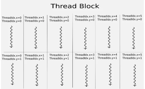
Thread. Athreadis the smallest computational unit in the CUDA programming model. At the time of execution, every thread will be assigned to one scalar processor. Also, each thread belongs to a thread block. Finally, each thread has a unique index inside its respective thread block, which depending on dimensions of the thread block can be

accessed via

1. threadIdx.x,

2. threadIdx.y (only if the thread belongs to a 2D or 3D thread block), 3. threadIdx.z (only if the thread belongs to a 3D thread block).

Thread block. A group of threads together form a thread block. Each thread block belongs to a grid. Finally, each thread block has a unique index inside its respective grid, which depending on the dimensions of the grid can be accessed via

1. blockIdx.x,

2. blockIdx.y (only if the thread block block belongs to a 2D or 3D grid), 3. and blockIdx.z(only if the thread block belongs to a 3D grid).

Figure 2.1 illustrates an example of a two dimensional thread block with 2 rows and 6 columns.

Figure 2.1: Example of a 2D thread block with 2 rows and 6 columns.

(21)

GPGPU computing 10

example of a two dimensional block with 2 rows and 4 columns.

Figure 2.2: Example of a 2D grid with 2 rows and 4 columns.

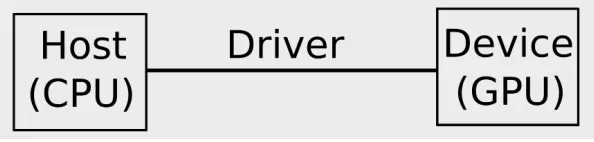
Kernel. At the time of execution, all threads in all thread blocks will run the same function. which is known as Kernel.

Device. In the CUDA programming model, device refers to the GPU that executes kernels on threads.

Host. In the CUDA programming model,hostrefers to the CPU that initializes kernels. Figure2.3 shows the relationship between the host and the device.

Figure 2.3: Host and device in the CUDA programming model.

Compute capability (CC). Every CUDA device is built on a core architecture with some specific capabilities. Each device is numbered by aCompute capability (CC), which is of the formA.B. This numbering makes it easier to distinguish architectures from each

other. In this presentation,A as the major part, specifies the architecture series, and B, as the minor part, relates to the special improvements to each architecture. For example, devices of compute capability 3.0, 3.1, and 3.2 have the same architecture core, however, they have different hardware optimizations.

Warp. Every 32 threads inside a thread block form a warp.

(22)

GPGPU computing 11

schedulers, and cache. At the time of execution, the device driver will assign each thread block to one streaming multiprocessor. After being scheduled by the warp scheduler,

each thread of the thread block will run the kernel on one processing core.

Warp scheduler. At the time of execution, each streaming multiprocessor partitions threads into warps. In the next step, warps will be scheduled by a warp scheduler for execution on scalar processors. Table2.1 shows the maximum number of warps that can reside on streaming multiprocessors of different compute capabilities.

Compute capability 1.0/1.1 1.2/1.3 2.x 3.x and higher

The maximum number of threads per SM 768 1024 1536 2048

The maximum number of warps 24 32 48 64

Table 2.1: The maximum number of warps per streaming multiprocessor.

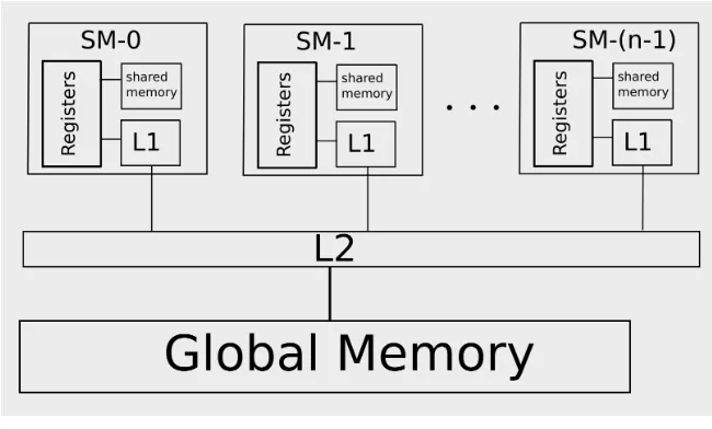
2.1.2 CUDA memory model

The CUDA platform has multiple levels of memory. As a programmer, it is critical to use different types of GPU memory properly. In other words, each level of GPU memory should be used for a specific type of application. Figure2.4shows levels of GPU memory for devices of compute capability 2.0 and higher.

Figure 2.4: CUDA memory hierarchy for CC 2.0 and higher.

(23)

GPGPU computing 12

Registers. Registers are fastest type of memory on GPUs. Accessing to a register has almost no cost, because it is placed on the streaming multiprocessor. Each streaming

multiprocessor has a limited number of registers. Table2.2shows the number of available registers on one streaming multiprocessor for CUDA-capable NVIDIA GPUs.

Compute capability 1.x 2.x 3.x 4.x 5.x 6.x The number of 32-bit registers/SM 124 63 255 255 255 255

Table 2.2: The number of 32-bit registers per streaming multiprocessor.

Global memory. This type of memory is available to all threads in all thread blocks.

Global memory is the slowest type of GPU memory.

Coalesced accesses to global memory. Inside a warp, consecutive threads can have access to consecutive words in global memory in acoalesced way. For doing so, the GPU driver translates multiple read or write memory calls into a single memory call. For

current CUDA-enabled GPUs,

L1 Cache. This type of on-chip GPU memory is accessible by all threads inside a warp. GPUs have comparably less amount of L1 cache per multiprocessor than CPUs have. Depending on the GPU architecture (CC), the programmer can enable or disable the L1

caching.

L2 Cache. This type of off-chip GPU memory is available on devices of compute capa-bility 2.0 and higher. If L1 cache is enabled, all read requests to global memory will first go through the L1 cache, and then through the L2 cache. However, if the L1 cache is disabled, all read transactions will go directly through the L2 cache.

Local memory. Each thread can have a private off-chip memory, known as local mem-ory. Local memory is allocated on global memory, therefore, accesses to local memory will be slow. However, accesses to local memory will be coalesced if adjacent threads of the same warp will have access to the same index of an array. Devices of compute capability 1.x have 16 KB of local memory. Finally, devices of other compute capabilities

have 512 KB of local memory.

Shared memory. This type of memory is available to all threads inside the thread block. It can be used

1. for communicating between threads inside the thread block, and

(24)

GPGPU computing 13

On the positive side, accesses to shared memory have almost no cost, because, compared to registers, it only takes a few more cycles. On the negative side, shared memory accesses

can go through bank conflicts, meaning that all accesses will be serialized.

Constant memory. This type of read-only memory is accessible to all threads of a grid and can be used for storing constant data. In order to use constant memory efficiently, all accesses should be to the same memory address at the same time. Otherwise, memory requests will be serialized. Currently, the total amount of constant memory for GPUs of

all compute capabilities is equal to 64 KB.

Texture memory. This is another type of read-only memory and similar to constant memory, can be used for storing constant data. However, unlike constant memory, scat-tered to constant memory will not be serialized.

2.1.3 Examples of programs in CUDA

In this section, we present two simple examples of programming in the CUDA-C/C++.

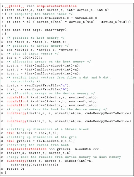
Simple vector addition in CUDA. Figure2.5 presents a pseudo-code for computing vector addition on GPUs in the following way:

1. First, the program allocates host memory for host a,host b as input array, and

for host c as the output array. (L16:L18)

2. The program reads input data from files into host a and host b, respectively (L21:L22).

3. In next step, the program allocatesdevicememory fordevice a,device b,device c

(L25:L27).

4. Then, the program copies input vectors from host memory to device memory. 5. The program sets dimensions of the thread block and grid block, respectively (L34

and L37).

6. At this point, the program invokes the CUDA kernel simpleVectorAddition (L40). 7. Now, inside the kernel, each thread computes its index with respect to its thread

block index and size of the thread block, and then, it computes the result of addition for two elements of the same relative index from each input array (L4:L5).

8. After completing the computation by the device, the program copies back the result of computation into the output array, host c (L44).

(25)

GPGPU computing 14

1 _ _ g l o b a l _ _ v o i d s i m p l e V e c t o r A d d i t i o n

2 ( int * d e v i c e _ a , int * d e v i c e _ b , int * d e v i c e _ c , int n )

3 { /* c o m p u t i n g the t h r e a d i n d e x */

4 int tid = b l o c k I d x . x * b l o c k D i m . x + t h r e a d I d x . x ;

5 if ( tid < n ) { d e v i c e _ c [ tid ] = d e v i c e _ b [ tid ] + d e v i c e _ a [ tid ];}

6 }

7 int m a i n ( int argc , c h a r ** a r g v ) 8 {

9 /* p o i n t e r s to h o s t m e m o r y */

10 int * host_a , * host_b , * h o s t _ c ; 11 /* p o i n t e r s to d e v i c e m e m o r y */

12 int * d e v i c e _ a , * d e v i c e _ b , * d e v i c e _ c ;

13 /* s i z e of i n p u t v e c t o r */ 14 int n = 1 0 2 4 * 1 0 2 4 ;

15 /* a l l o c a t i n g a r r a y s on the h o s t m e m o r y */

16 h o s t _ a = ( int *) m a l l o c ( s i z e o f ( int ) * n ) ; 17 h o s t _ b = ( int *) m a l l o c ( s i z e o f ( int ) * n ) ;

18 h o s t _ c = ( int *) m a l l o c ( s i z e o f ( int ) * n ) ;

19 /* r e a d i n g i n p u t v e c t o r s f r o m f i l e s a . dat and b . dat ,

r e s p e c t i v e l y . */

20 h o s t _ a = r e a d I n p u t F r o m F i l e (" a ") ;

21 h o s t _ b = r e a d I n p u t F r o m F i l e (" b ") ;

22 /* a l l o c a t i n g a r r a y s on the d e v i c e m e m o r y */

23 c u d a M a l l o c( ( v o i d **) & d e v i c e _ a , n * s i z e o f ( int ) ) ;

24 c u d a M a l l o c( ( v o i d **) & d e v i c e _ b , n * s i z e o f ( int ) ) ; 25 c u d a M a l l o c( ( v o i d **) & d e v i c e _ c , n * s i z e o f ( int ) ) ;

26 /* c o p y d a t a f r o m the h o s t to the d e v i c e m e m o r y */

27 c u d a M e m c p y( d e v i c e _ a , a , s i z e o f ( int ) * n , c u d a M e m c p y H o s t T o D e v i c e )

;

28 c u d a M e m c p y( d e v i c e _ b , b , s i z e o f ( int ) * n , c u d a M e m c p y H o s t T o D e v i c e ) ;

29 // s e t t i n g up d i m e n s i o n s of a t h r e a d b l o c k

30 d i m 3 b l o c k D i m = (512 ,1 ,1) ;

31 // s e t t i n g up d i m e n s i o n s of the g r i d 32 d i m 3 g r i d D i m = ( n / b l o c k D i m . x ,1 ,1) ; 33 // i n v o k i n g the k e r n e l f r o m h o s t

34 s i m p l e V e c t o r A d d i t i o n < < < gridDim , b l o c k D i m > > > 35 ( d e v i c e _ a , d e v i c e _ b , d e v i c e _ c , n ) ;

36 // c o p y b a c k the r e s u l t s f r o m d e v i c e m e m o r y to h o s t m e m o r y

37 c u d a M e m c p y( host_c , d e v i c e _ c , s i z e o f ( int ) * n ,

c u d a M e m c p y D e v i c e T o H o s t ) ;

38 r e t u r n 0;

39 }

(26)

GPGPU computing 15

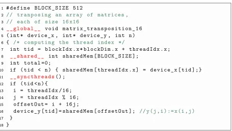
1 # d e f i n e B L O C K _ S I Z E 512

2 // t r a n p o s i n g an a r r a y of m a t r i c e s ,

3 // e a c h of s i z e 16 x16

4 _ _ g l o b a l _ _ v o i d m a t r i x _ t r a n s p o s i t i o n _ 1 6

5 ( int * d e v i c e _ x , int * d e v i c e _ y , int n )

6 { /* c o m p u t i n g the t h r e a d i n d e x */

7 int tid = b l o c k I d x . x * b l o c k D i m . x + t h r e a d I d x . x ;

8 _ _ s h a r e d _ _ int s h a r e d M e m [ B L O C K _ S I Z E ];

9 int t o t a l =0;

10 if ( tid < n ) { s h a r e d M e m [ t h r e a d I d x . x ] = d e v i c e _ x [ tid ];}

11 _ _ s y n c t h r e a d s() ;

12 if ( tid < n ) {

13 i = t h r e a d I d x / 1 6 ;

14 j = t h r e a d I d x % 16;

15 o f f s e t O u t = i + 16 j ;

16 d e v i c e _ y [ tid ]= s h a r e d M e m [ o f f s e t O u t ]; // y ( j , i ) := x ( i , j )

17 }

18 }

Figure 2.6: A CUDA example for transposing matrices by using shared memory.

size n, our example computes transposition for n/256 matrices. We assume that the kernel configuration is similar to that of the previous example. This kernel computes the transposition in the following way.

1. Each thread computes its index with respect to its thread block index and size of the thread block (L7).

2. In the next step, a shared array of size BLOCK SIZE is allocated for all threads of the thread block (L8).

3. Then, each thread reads its corresponding value from the input vector into its respective shared memory address (L10).

4. The barrier syncthreads() synchronizes all threads of the thread block (L11). 5. At this step, each thread computes the row number and the column number of its

corresponding value in the input vector, namely, (i, j) (L13 and L14).

6. In the next step, each thread computes the offset for its corresponding memory address in output vector, namely, (j, i) (L15).

7. Finally, each thread writes its corresponding value to the output vector (L16).

(27)

GPGPU computing 16

2.1.4 Performance of GPU programs

Bandwidth. Bandwidth refers to the rate of transferring data between two memory

addresses (that might be in different levels). Theoretical bandwidth is the maximum value for the GPU memory bandwidth which can be calculated by BT =f×w×2 with

1. f as the clock frequency of the GPU memory, and

2. w as the width of memory interface (in terms of number of bytes).

For example, for a GPU memory with the clock rate of 1 GHZ and the memory interface of 384 bits wide, we have

BT = 1×109×

384

8 ×2 = 96 GB/s.

Practical bandwidth. Practical (effective) bandwidth is the bandwidth that can be achieved on a GPU in practice. Practical bandwidth can be computed by

BE =

(dr+dw)

t (2.1)

where

1. dr is the amount of data that is being read from the memory,

2. dw is the amount of data that is written to the memory, and

3. t is the elapsed time for reading from the memory and writing to the memory.

For example, if the program spends 4 milliseconds for copying a vector of N = 220 _long

integers (each of size of 8 machine-words) to another vector, then effective bandwidth is

BE =

((220_×₈_×₈₎_×₂₎

(4×10−3₎ = 33.5 GB/s.

Value of practical bandwidth is always less than the value of theoretical bandwidth. Also, enabling some error correction features (like Error-Correcting-Code in NVIDIA cards) can further reduce the effective bandwidth.

Occupancy. Occupancy refers to the ratio of the total number of running warps to the maximum number of warps that can be concurrently executed on each streaming multiprocessor. Following factors can affect the percentage of achieved occupancy:

1. the amount of shared memory per each streaming multiprocessor, 2. the number of registers per each thread,

(28)

GPGPU computing 17

4. the size of a thread block (which we would prefer to be a multiple of 32).

Data latency. This term refers to the time spent between requesting the data by a warp and when the data is ready to be processed by the warp. During this time, the warp scheduler executes another warp, therefore, the requesting warp should be waiting. We try to hide the data latency by increasing the occupancy percentage.

Register spilling. As long as there are enough registers left to be allocated, single variables and constant values will always be stored in registers. However, an array inside a thread will not always be stored in registers. In fact, the compiler makes the decision to store an array in registers of the streaming multiprocessor only if the following conditions are met:

- the compiler should be able to determine the indexes of the array, and - there should be enough number of registers to allocate to the array.

Otherwise, the array will be stored in local memory, which will result inregister spilling. As we explained before, accesses to local memory is costly, therefore, register spilling will have a negative impact on the memory bandwidth. Also, even if the register spilling does not happen, allocating too many registers to each thread will lower the number of concurrent warps, and consequently, will lower the overall occupancy of the application.

Shared memory bank conflicts. Shared memory is divided into partitions of the same size, namely, shared memory banks. The default size of a shared memory bank is 32 bits, however, for devices of compute capability 2.0 and higher, size of shared memory banks can be configured to 64 bits. Inside a warp, multiple accesses to the same address of shared memory will result in shared memory bank conflicts. As a result, conflicted accesses will be serialized, and therefore, will lower the bandwidth.

Arithmetic bound kernels. Arithmetic bound kernels spend most of the computation time for issuing arithmetic instructions. In other words, performance is limited by the high number of arithmetic instructions that should be issued at each clock cycle. For an arithmetic bound kernel, we would prefer to lower warp divergence and therefore, avoid using if-else statements as much as possible. Also, we can balance the computation among arithmetic units of each streaming multiprocessor. For example, we can compute part of the integer arithmetic to the floating point arithmetic units and Special Function Units (SFUs).

(29)

GPGPU computing 18

An effective solution for increasing performance of memory bound kernels is to make sure the data latency is minimized and more warps will be concurrently executed. In other

words, occupancy should be increased to hide the latency. Also, we must ensure that accesses to global memory are minimized by

1. storing data in a data structure that facilitates coalesced accesses, and 2. (if possible) reusing the same data for more computations.

As a final note, for a memory bound GPU kernel, the practical bandwidth is usually close to the peak of the theoretical bandwidth.

Arithmetic intensity. Arithmetic intensity is defined as the ratio of the number of arithmetic instructions to the total amount of processed data. More importantly, this term does not have a unique definition. For example, we can define the total amount of processed data

1. as the total number of memory instructions, or 2. as the amount of data in terms of bytes.

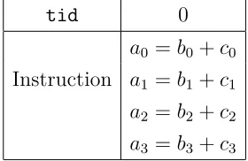
Instruction level parallelism (ILP). This term refers to the parallelization of

in-dependent instructions at the level of hardware. For example, assume that ai, bi, ci

(0≤i <4) are pointers to non-overlapping addresses in the memory. Then, as shown in Figure2.7, we can concurrently compute 4 additions ai :=bi+ci by using 4 threads.

tid 0 1 2 3

Instruction a0 =b0+c0 a1 =b1+c1 a2 =b2+c2 a3 =b3+c3

Figure 2.7: Four independent instructions.

On the other hand, as shown in Figure2.8, one thread can be used for computing all four additions. However, in practice, it is very difficult to exploit the ILP, mostly because the programmer does not have direct control over it. In fact, it is the compiler that makes the decision for using ILP. Depending on the architecture of the device, 2 or 4 instructions

(30)

GPGPU computing 19

tid 0

a0 =b0+c0

Instruction a1 =b1+c1

a2 =b2+c2

a3 =b3+c3

Figure 2.8: An example of ILP.

2.1.5 Profiling CUDA applications

Profiler. A profiler is software that is used for inspecting the performance of an ap-plication. As part of the software development kit (CUDA-SDK), NVIDIA corporation

provides nvprof as the official command-line profiler for CUDA applications. In next step, we explain a number of the most important metrics that can be measured by this profiler. Moreover, Table 2.3 shows a list of the nvprof metrics that will be used for measuring the performance of our implementation.

Instruction per cycle (IPC). This metric measures the total number of instructions

that are issued on each streaming multiprocessor at each clock cycle.

Achieved occupancy. This metric represents the ratio of the total number of run-ning warps to the maximum possible number of the warps that can be executed on the multiprocessor.

Instruction replay overhead. This metric represents the following ratio:

N(issued)−N(requested)

N(requested)

(2.2)

where:

1. N(issued) is the total number of issued instructions, and

2. N(requested) is the total number of requested instructions.

There are similar ”replay overhead” metrics for some other instructions, for example, global memory replay overhead and shared memory replay overhead measure overheads of global memory and shared memory instructions, respectively.

(31)

GPGPU computing 20

DRAM read and write throughput. This metric measures the memory throughput for memory read transactions between the device memory and the L2 cache.

Metric name description

achieved occupancy Percentage of occupancy for all SMs

ipc Instruction per cycle

gst throughput Global memory store throughput

gld throughput Global memory load throughput

gst efficiency Global memory store efficiency

dram utilization Device memory utilization (a value between 0 and 10)

Table 2.3: A short list of performance metrics of nvprof.

2.1.6 A note on psuedo-code.

We present our algorithms in pseudo-codes similar to the CUDA programming model.

Host functions. Name of this type of function begins with the keyword Host. Host functions can only be called from the host (CPU). Moreover, this type of function are used for

1. initializing the input data, and 2. invoking GPU kernels.

Kernel functions. The name of this type of function begins with the keyword Kernel.

Kernel functions will be loaded on each streaming multiprocessor, then, all threads will execute the same code. Kernel functions can only be called from host functions. Fi-nally, this type of function never returns any values, instead, they only depend on global memory for communicating to the host.

Device functions. The name of this type of function begins with the keyword Device.

Device functions can only be called from kernel functions. However, device functions can return values to their invoker kernel.

Size of a machine-word. We assume that a machine-word (register) is 64-bits wide.

Fortran style arrays. In this thesis, we present arrays in the following way:

1. ~x refers to vector of digits, each of size of of a machine-word, 2. ~x[i] refers to i-th digit of ~x, and

(32)

Fast Fourier Transforms 21

2.2 Fast Fourier Transforms

In this section, we review the Discrete Fourier Transform over a finite field, and its related concepts.

Primitive and principal roots of unity. Let R be a commutative ring with units. Let N >1 be an integer. An elementω∈ Ris aprimitiveN-th root of unity if for 1< k≤N we haveωk_{= 1} _⇐⇒ _k ₌_N_{. The element}_ω _{∈ R} _{is a} _principal _N_{-th root of unity if}

ωN _{= 1 and for all 1} _≤_{k < N} _{we have}

N−1

X

j=0

ωjk = 0. (2.3)

In particular, ifN is a power of 2 andωN/2 =−1, thenωis a principalN-th root of unity. The two notions coincide in fields of characteristic 0. For integral domains every primitive root of unity is also a principal root of unity. For non-integral domains, a principalN-th root of unity is also a primitive N-th root of unity unless the characteristic of the ring R is a divisor ofN.

The discrete Fourier transform (DFT). Let ω ∈ R be a principal N-th root of unity. TheN-point DFT at ω is the linear function, mapping the vector~a= (a0, . . . , aN−1)T to

~b= (b0, . . . , bN−1)T by~b = Ω~a, where Ω = (ωjk)0≤j,k≤N−1. If N is invertible in R, then

the N-point DFT at ω has an inverse which is 1/N times the N-point DFT at ω−1_.

The fast Fourier transform. Letω∈ R be a principalN-th root of unity. Assume that N can be factorized toJ K withJ, K > 1. Recall Cooley-Tukey factorization formula [6]

DFTJ K = (DFTJ ⊗IK)DJ,K(IJ ⊗DFTK)LJ KJ , (2.4)

where, for two matricesA, B overRwith respective formats m×n and q×s, we denote byA⊗B anmq×nsmatrix over R called the tensor product ofA byB and defined by

A⊗B = [ak`B]k,` with A= [ak`]k,` (2.5)

In the above formula, DFTJ K, DFTJ and DFTK are respectively the N-point DFT at

ω, the J-point DFT at ωK _{and the} _{K-point DFT at} _ωJ_{. The} _{stride permutation matrix}

LJ K_J permutes an input vector x of lengthJ K as follows

(33)

for all 0 ≤ j < J, 0 ≤ i < K. If x is viewed as an K ×J matrix, then LJ K

J performs a

transposition of this matrix. The diagonal twiddle matrix DJ,K is defined as

DJ,K = J−1

M

j=0

diag(1, ωj, . . . , ωj(K−1)), (2.7)

Formula (2.4) implies various divide-and-conquer algorithms for computing DFTs effi-ciently, often refered as fast Fourier transforms (FFTs). See the seminal papers [20] and [11] by the authors of the SPIRAL abd FFTW projects, respectively. This formula also implies that, if K divides J, then all involved multiplications are by powers of ωK_.

In the factorization of the matrix DFTJ K, viewing the sizeK as a base case and assuming

thatJ is a power ofK, Formula (2.4) translates into Algorithm2.1. In this algorithm, as in the sequel of this section, ω ∈ R be a principal N-th root of unity and (α0α1...αN−1)

(34)

Algorithm 2.1 Radix K Fast Fourier Transform in R procedure FFTradix K((α0α1...αN−1), ω,N =J·K)

for 0≤j < J do . Data transposition

for 0≤k < K do γ[j][k] := αkJ+j end for

end for

for 0≤j < J do . Base case FFTs

c[j] := FFTbase−case(γ[j], ωJ, K)

end for

for 0≤k < K do . Twiddle factor multiplication for 0≤j < J do

δ[k][j] :=c[j][k]∗ωjk end for

end for

for 0≤k < K do .Recursive calls

δ[k] = FFTradix K(δ[k], ωK, J) end for

for 0≤k < K do . Data transposition

for 0≤j < J do α[jK+k] := δ[k][j]

end for

return(α0α1...αN−1)

end procedure

The recursive formulation of Algorithm 2.1 is not appropriate for generating code tar-geting many-core GPU-like architectures for which, formulating algorithms iteratively

facilates the division of the work into kernel calls and thread-blocks.

(35)

Chapter 3 Arithmetic Computations Modulo

Sparse Radix Generalized Fermat

Numbers

The n-th Fermat number, denoted by Fn, is given by Fn = 22

n

+ 1. This sequence plays an important role in number theory and, as mentioned in the introduction, in the development of asymptotically fast algorithms for integer multiplication [21,13].

Arithmetic operations modulo a Fermat number are simpler than modulo an arbitrary positive integer. In particular 2 is a 2n+1-th primitive root of unity modulo Fn.

Unfor-tunately, F4 is the largest Fermat number which is known to be prime. Hence, when

computations require the coefficient ring be a field, Fermat numbers are no longer inter-esting. This motivates the introduction of other family of Fermat-like numbers, see, for instance, Chapter 2 in the text book Guide to elliptic curve cryptography [14].

Numbers of the form a2n +b2n where a > 1, b ≥ 0 and n ≥ 0 are called generalized Fermat numbers. An odd prime p is a generalized Fermat number if and only if p is congruent to 1 modulo 4. The case b = 1 is of particular interest and, by analogy with the ordinary Fermat numbers, it is common to denote the generalized Fermat number a2n

+ 1 byFn(a). So 3 is F0(2). We calla the radixofFn(a). Note that, Landau’s fourth

problem asks if there are infinitely many generalized Fermat primes Fn(a) withn >0.

In the finite ring _Z/Fn(a)Z, the elementa is a 2n+1-th primitive root of unity. However,

when using binary representation for integers on a computer, arithmetic operations in

Z/Fn(a)Z may not be as easy to perform as in Z/FnZ. This motivates the following.

(36)

Representation of_Z/p_Z 25

Definition 1 We call sparse radix generalized Fermat number, any integer of the form

Fn(r) where r is either 2w + 2u or 2w −2u, for some integers w > u≥0. In the former case, we denote Fn(r) by Fn+(w, u) and in the latter by Fn−(w, u).

Table 3.1 lists a few sparse radix generalized Fermat numbers (SRGFNs, for short) that are prime. For each p among those numbers, we give the largest power of 2 dividing

p−1, that is, the maximum length N of a vector to which a radix-K FFT algorithm (like Algorithm2.1) whereK is an appropriate power of 2.

p max{2e _s.t.₂e _| _p₋₁_}

(263+ 253)2+ 1 2106 (264₋₂50₎4_{+ 1} ₂200

(263_{+ 2}34₎8_{+ 1} ₂272

(262_{+ 2}36₎16_{+ 1} ₂576

(262+ 256)32+ 1 21792 (263₋₂40₎64_{+ 1} ₂2500

(264₋₂28₎128_{+ 1} ₂3584

Table 3.1: SRGFNs of practical interest.

Notation 1 In the sequel of this section, we consider p = Fn(r), a fixed SRGFN. We

denote by2e the largest power of 2dividingp−1and we define k = 2n, so thatp=rk+ 1

holds.

As we shall see in the sequel of this section, for any positive integer N which is a power

of 2 such that N divides p−1, one can find an N-th primitive root of unity ω ∈_Z/p_Z such that multiplying an element a ∈ _Z/p_Z by ωi(N/2k) for 0 ≤ i < 2k can be done in linear time w.r.t. the bit size of a. Combining this observation with an appropriate factorization of the DFT transform on N points over _Z/p_Z, we obtain an efficient FFT algorithm over_Z/p_Z.

3.1 Representation of

_Z

/p

_Z

We represent each elementx∈_Z/p_Zas a vector~x= (xk−1, xk−2, . . . , x0) of lengthk and

with non-negative integer coefficients such that we have

x ≡ xk−1rk−1+xk−2rk−2+· · ·+x0 mod p. (3.1)

This representation is made unique by imposing the following constraints

(37)

Representation of _Z/p_Z 26

2. or 0≤xi < r for all i= 0, . . . , (k−1).

We also map x to a univariate integer polynomial fx ∈ Z[T] defined by fx = Pk−i=01 xiti

such that x ≡ fx(r) mod p.

Now, given a non-negative integer x < p, we explain how the representation ~x can be computed. The case x = rk _{is trivially handled, hence we assume} _{x < r}k_{. For a}

non-negative integer z such that z < r2i

holds for some positive integer i ≤n = log₂(k), we denote by vec(z, i) the unique sequence of 2i _{non-negative integers (z}

2i₋₁, . . . , z₀) such

that we have 0≤zj < rand z =z2i₋₁r2 i₋₁

+· · ·+z0. The sequence vec(z, i) is obtained

as follows:

1. if i= 1, we have vec(z, i) = (q, s),

2. if i >1, then vec(z, i) is the concatenation of vec(q, i−1) followed by vec(s, i−1),

whereq ands are the quotient and the remainder in the Euclidean division of z byr2i−1. Clearly, vec(x, n) =~x holds.

We observe that the sparse binary representation of r facilitates the Euclidean division

of an non-negative integer z by r, when performed on a computer. Referring to the notations in Definition 1, let us assume that r is 2w + 2u, for some integers w > u ≥0. (The case 2w−2u would be handled in a similar way.) Let zhigh and zlow be the quotient

and the remainder in the Euclidean division of z by 2w. Then, we have

z = 2wzhigh+zlow = r zhigh+zlow−2uzhigh. (3.2)

Lets =zlow+−2uzhigh and q =zhigh. Three cases arise:

(S1) if 0≤s < r, then q and s are the quotient and remainder of z byr,

(S2) if r ≤ s, then we perform the Euclidean division of s by r and deduce the desired quotient and remainder,

(S3) if s <0, then (q, s) is replaced by (q+ 1, s+r) and we go back to Step (S1).

Since the binary representations of r2 _{can still be regarded as sparse, a similar procedure}

(38)

Finding primitive roots of unity in _Z/p_Z 27

3.2 Finding primitive roots of unity in

_Z

/p

_Z

Notation 2 Let N a power of 2, say 2`_{, dividing} _p₋₁ _{and let} _g _∈

Z/pZ be a N-th primitive root of unity.

Recall that such anN-th primitive root of unity can be obtained by a simple probabilistic procedure. Write p =qN + 1. Pick a random α ∈_Z/p_Z and let ω = αq_{. Little Fermat}

theorem implies that eitherωN/2 _{= 1 or}_ωN/2 ₌₋_{1 holds. In the latter case,}_ω _{is an}_N_-th

primitive root of unity. In the former, another random α ∈_Z/p_Z should be considered. In our various software implementation of finite field arithmetic [16,3,15], this procedure finds an N-th primitive root of unity after a few tries and has never been a performance bottleneck.

In the following, we consider the problem of finding an N-th primitive root of unity ω such thatωN/2k₌_r _{holds. The intention is to speed up the portion of FFT computation}

that requires to multiply elements of_Z/p_Z by powers ofω.

Proposition 1 In_Z/p_Z, the element r is a 2k-th primitive root of unity. Moreover, the

following algorithm computes an N-th primitive root of unity ω ∈ _Z/p_Z such that we

have ωN/2k=r in _Z/p_Z.

Algorithm 3.1 PrimitiveN-th rootω ∈_Z/pZ s.t. ωN/2k=r procedure PrimitiveRootAsRootOf(N, r, k, g)

α:=gN/2k

β :=α j := 1

whileβ 6=r do β :=αβ j :=j+ 1

end while

ω:=gj return(ω) end procedure

Proof Since gN/2k _{is a 2k-th root of unity, it is equal to} _ri0 _(modulo _{p) for some}

0≤i0 <2k wherei0 is odd. Let j be an non-negative integer. Observe that we have

Fast Fourier Transforms over Prime Fields of Large Characteristic and their Implementation on Graphics Processing Units

Scholarship@Western

Scholarship@Western

Fast Fourier Transforms over Prime Fields of Large Characteristic

Fast Fourier Transforms over Prime Fields of Large Characteristic

and their Implementation on Graphics Processing Units

and their Implementation on Graphics Processing Units

Abstract

Acknowlegements

Contents

List of Algorithms

List of Figures

List of Tables

Chapter 1

Introduction

Chapter 2

Background

2.1

GPGPU computing

2.1.1

CUDA programming model

2.1.2

CUDA memory model

2.1.3

Examples of programs in CUDA

2.1.4

Performance of GPU programs

2.1.5

Profiling CUDA applications

2.1.6

A note on psuedo-code.

2.2

Fast Fourier Transforms

Chapter 3

Arithmetic Computations Modulo

Sparse Radix Generalized Fermat

Numbers

3.1

Representation of

Z

/p

Z

3.2

Finding primitive roots of unity in

Z

/p

Z

_Z

_Z

_Z

_Z