F U L L P A P E R
Open Access
Inverting magnetic meridian data using
nonlinear optimization
Martin Connors
1*and Gordon Rostoker
2Abstract
A nonlinear optimization algorithm coupled with a model of auroral current systems allows derivation of physical parameters from data and is the basis of a new inversion technique. We refer to this technique as automated forward modeling (AFM), with the variant used here being automated meridian modeling (AMM). AFM is applicable on scales from regional to global, yielding simple and easily understood output, and using only magnetic data with no assumptions about electrodynamic parameters. We have found the most useful output parameters to be the total current and the boundaries of the auroral electrojet on a meridian densely populated with magnetometers, as derived by AMM. Here, we describe application of AFM nonlinear optimization to magnetic data and then describe the use of AMM to study substorms with magnetic data from ground meridian chains as input. AMM inversion results are compared to optical data, results from other inversion methods, and field-aligned current data from AMPERE. AMM yields physical parameters meaningful in describing local electrodynamics and is suitable for ongoing monitoring of activity. The relation of AMM model parameters to equivalent currents is discussed, and the two are found to compare well if the field-aligned currents are far from the inversion meridian.
Keywords:Current systems; Substorms; Geophysical inversion techniques; Nonlinear optimization; Geomagnetism;
Equivalent current
Background
The interpretation of ground magnetic data has long been realized as having an important role in understand-ing physical processes in near-Earth space. Much of the signal arises from electric currents in the ionosphere and flowing along magnetic field lines. An ideal inver-sion method would allow the characteristics of these currents to be found at any time, reflecting physical vari-ations in near-Earth electrodynamics.
Methods such as that of Kamide, Richmond, and Matsushita (called KRM) (Ahn et al. 1995) and assimi-lative modeling of ionospheric electrodynamics (AMIE) (Richmond 1992) allow determination of electrodynamic quantities of the upper atmosphere, and models exist for the entire near-Earth system with input from the solar wind (Ridley et al. 2002). These models incorporate aur-oral and magnetospheric physics in ways which are linked to the inversion in a complex way. The KRM and AMIE
techniques are based on a global representation of electric and magnetic fields related through electric currents and conductivities. The latter parameter in particular is diffi-cult to determine, although AMIE attempts to refine it through the ingestion of many types of data. A simpler approach, which does not require a global representation, can be given through direct application of the Biot-Savart integral to a specified configuration of electric currents in space and the ionosphere, with corrections for Earth con-ductivity. Specifying where the currents flow constitutes making a forward model, and the parameters of this model can be adjusted to obtain a best fit to data. If an ac-ceptable fit is attained, one can claim that the configur-ation of electric currents usefully represents the physical current system. This simpler approach was implemented using an optimization procedure and referred to as auto-mated forward modeling (AFM), by Connors (1998).
Within the more general context of magnetic data inver-sion, AFM would be considered to be“parametric inver-sion” (Li and Oldenburg 1996). Parametric inversion requires simple causation and “a great deal of a priori knowledge.”In the case of auroral zone currents, desirable
* Correspondence:[email protected] 1
Athabasca University Observatories, 1 University Drive, Athabasca, AB T9S 3A3, Canada
Full list of author information is available at the end of the article
physical quantities would be, for example, the current strength and latitudinal location of the auroral electrojets. These are useful parameters to allow computation of a model, and they clearly correspond, at least at some level of approximation, to physical quantities, based on long-standing (Boström 1964) knowledge. Here, we describe a new method of optimizing a simple forward model involv-ing auroral zone currents, includinvolv-ing field-aligned currents (FACs), for inversion of magnetic data alone, without the use of electrodynamic quantities such as conductivity. We give examples of use of this technique for simple models of electrojets over meridians and refer to this restricted form of use as automated meridian modeling (AMM). Connors et al. (2014) used a similar approach (the same computer code with a more general forward model and constraints) to deduce parameters for the substorm current wedge, using data from the North American re-gion, and compare them to those inferred using an inde-pendent space-based dataset. We usually refer to the technique used and cursorily described in supplemental material, by Connors et al. (2014) as automated regional modeling (ARM), and explain below its relation to the present work.
The thrust of this study is to automate forward model-ing techniques, most particularly those based on direct precision integration of the Biot-Savart integral. The pa-rameters are physically meaningful variables, and their variation is taken to indicate physical changes respon-sible for the observed perturbations dB. In practice, the parameters used are simple geometric ones and the current. The method is thus complementary to other methods such as KRM and AMIE that necessitate in-volvement of electrodynamic parameters such as the conductivity. That the interplay of parameters involved in more complex models can lead to a possible reduc-tion in their physical meaning has been discussed by Ridley et al. (2002). The fact that ground magnetic data cannot be reproduced well by current MHD models sup-plying boundary conditions to AMIE has also been dis-cussed (Ridley et al. 2001). In our technique, the primary condition is a good match of optimized forward model output to ground magnetic data, and physical assump-tions are kept to a minimum.
Regional techniques with some resemblance to AFM have already been developed but generally use a simpler magnetic field model than we do. Lühr et al. (1994) de-veloped an automated fitting routine to optimize param-eters for simple current systems consisting of a line current, a strip of constant east–west current density, or a region in which the east–west current density varied as a quadratic (parabolic model). The current densities obtained from optimizing the models using the Mar-quardt technique (very similar to that used in this study) were compared with those obtained by the EISCAT
radar. The current density estimated from the ground was found to be about 15 % higher than that derived from the radar (and in two cases rocket) measurements. The discrepancy was attributed to induction effects. An-other technique based on line currents and a flat Earth was developed by Popov et al. (2001). At any given time, this technique gives a profile of current density, and total current across the meridian can also be deter-mined. Earth induction is taken into account. Presenta-tion of the data for a day allows contour plots to be made showing the changes in the patterns of current density. Our focus differs in that we aim for the simplest possible parameters in order to eventually compare them with each other and with outside factors. Since our pa-rameters imply simple causation and are based on a priori knowledge, we consider the optimized forward model to represent data inversion in the sense of Li and Oldenburg (1996). We now proceed to discuss our method in detail and then give examples in which the output parameters are useful in understanding auroral events.
Methods
Here, we describe first how magnetic perturbations due to electric current systems in near-Earth space may be calculated to form a forward model. Next, the general techniques of optimization that allow automation of the modeling procedure are described. This is followed by a description of constraints and weighting that allow use of AFM on global, regional, or local scales. Finally, we describe local application to auroral electrojets as used in the data analysis part of the paper below.
Magnetic field model
Methods for calculating the perturbations due to physic-ally realistic current systems were presented by Kisabeth (1972). He proposed combinations of those current sys-tems which reproduced the input data. The data were most often in the form of perturbations observed along meridian chains of magnetometers. The proposed current systems constitute a forward model, and if the perturbations they produce agree with the data, confi-dence can be placed in the physical parameters of the model. Kisabeth and Rostoker (1977) performed studies of electrojets using these techniques. Kisabeth (1979) de-veloped several methods of resolving the Biot-Savart inte-gral that could be employed depending on circumstances, and Earth induction was included in the models. In this early forward modeling approach, determination of pa-rameters was done manually. In practice, and partly due to limitations of the manual approach, application of for-ward modeling to complex situations involving arbitrary distributions of stations has been difficult. An element of
was involved. In complex situations, the number of pa-rameters involved became large, and their determination from data at the many stations needed to uniquely optimize them became problematic. An automated tech-nique for finding an optimal set of parameters for model-ing magnetic data is needed.
The meaning of the word“optimal”is that a set of pa-rameters in the forward model has been changed (pos-sibly) from initial values guessed at, to improve the model’s representation of data. The deviation of a scalar model F from a scalar data at a set of N observation points xi may be represented by the scalar value
chi-squared χ2¼X
parameters in the model, andσian error value applicable for each measurement. In geomagnetism, the observa-tions are usually along three orthogonal axes, X being northward, Y being eastward, and Z being downward. TheX andYdirections are usually with respect to mag-netic north (usually local magmag-netic as determined at the time of instrument installation). In some cases, for example permanent observatories, measurements are done in the geodetic system, and if there is a significant deviation between magnetic and geodetic north (i.e., declination), such observations should be rotated into a geomagnetic coordinate system (Untiedt and Baumjohann 1993). Also, the squared separation in a vector space with three dimensions is the sum of the squares of separations along the orthogonal axes, so one can simply express the chi-squared for magnetic measurements as
χ2¼XN
where subscripts corresponding to the axes have been added to the measurement, model, and error values. In some fields where a modeling approach is applied, errors may be rigorously determined, but it is usually the case in geomagnetism that instrumental error is small, so that most of the error arises from the model not being able to completely represent the data. Setting a large error value for a certain station’s data is equivalent to applying a small weighting to it in the sum. The geometry of the χ2
space, path to optimization, and possibly the final re-sult are all affected by the weightings. Standard methods of applying weightings define classes of AFM, and the weightings are not changed during a run. Application of weightings is a standard practice in geophysical data in-version, often done to reduce dominant sources that can mask an overall signal (Li and Oldenburg 1996). Calcula-tion of equivalent currents often is based on only the
horizontal components of the surface magnetic field (Untiedt and Baumjohann 1993), and this corresponds to applying zero weight (in the view above, infinite error) to the vertical component. Explicit or implicit use of weighting functions that vary by component, as here, is an established practice, and details of its implementation in AFM will be given below.
Optimization of parameters
Parameters of a linear model can be optimized in one step that minimizes the squared (and perhaps weighted) deviation,χ2, but in nonlinear cases such as those arising in magnetic problems, the minimization equations are generally not analytically soluble. Solution requires nu-merically following gradients of χ2 in the parameter space. The Levenberg-Marquardt method is now widely used for such problems. It “works very well in practice and has become the standard”(Press et al. 1992, p. 683). It is a variable metric method that attempts to find an optimal step size in parameter space and is related to Newton’s method in the sense of following gradients to-ward a solution but enhanced in the region of a mini-mum by a quadratic approach. Details of the algorithm are given by Press et al. (1992) and by Lampton (1997). A brief description is also given by Lühr et al. (1994). As in that study, theYor eastward magnetic component is not normally used in our meridian chain inversions. The option exists to include it, however, for example in re-gional applications (such as ARM) rather than on a me-ridian. Since our technique includes a weighting applied to any component of data from any station, suppression or inclusion of effects from the Ycomponent is readily done by changing its weighting.
Levenberg-Marquardt method
We assume that χ2 for a forward model can be repre-sented in the space of its parameters as a differentiable function. This is the case for magnetic field models if usingM physically meaningful parameters, which define a space within which we denote those parameters by a vector a. The χ2 function can be expanded about any point a0 in this parameter space of M dimensions, to
have a value at another pointa(i.e., for a different set of parameters) which is
χ2ð Þ≈χa 2 a is the so-called Hessian matrix. The truncated expansion is a quadratic form. If the gradient is set to zero and the pointa0is thus regarded as the extremal point, Newton’s method simply givesA(a−a0) =b, with solutiona = a0+
A−1b. This solution is to be regarded in an iterative sense, since the Hessian matrix and the gradient vector b are both evaluated at the expansion point and may not be rep-resentative of the behavior of theχ2function all the way to its extremum. If necessary, as is generally the case in modeling magnetic fields, the derivatives can be evaluated numerically. If one is far from the extremum, linear terms will dominate. Then, the gradient can be followed down-slope toward the minimum. The problem with this ap-proach is that one does not know how far to follow the gradient. The Levenberg-Marquardt process attempts to solve this problem by combining use of the quadratic form near the extremum of χ2with following a gradi-ent, including a self-correcting method of determining how far to follow it. The modified system A′(a−a0) =
bcontains the desired solution, with A′ij¼Aij1þλδij the elements of the new combined matrix A′andδthe identity matrix. The parameter λ is an effective scale length and is modified as the solution progresses, to move most efficiently toward the minimum. For λ= 0, we recover the quadratic approach, while if λ is very large, A′ becomes diagonally dominant and the linear case is effectively in force. Ultimately, in the case of successful approach to an extremum, the value of λ is reduced to near zero, the pure quadratic form appro-priate to being near a minimum is used, and conver-gence accelerates. Based on these observations, the
“recipe” for the Levenberg-Marquardt technique given by Press et al. (1992), p. 684, may be used. An opti-mal starting value of λ must be determined by the user. The recipe is:
1. For a starting guess at the parametersa0, compute χ2
minimum and must increaseλsignificantly (they suggest a factor of 10) and repeat step 3.
5. Ifχ2(a) <χ2(a0), one is nearer to the minimum, soa
is a better guess thana0. One must replacea0in
step 3 bya, decreaseλto reflect being nearer the minimum, and redo step 3.
Steps 4 and 5 must include some criterion to deter-mine when iteration is complete. This may be by track-ing of successive values of χ2 so that when it stops changing much, one stops. While this is a desirable ap-proach, it is more practical simply to count and limit the number of iterations. This should be coupled with exam-ination of output at each step so that the behavior of χ2 is monitored and can be seen to be reasonable.
Variants in automated forward modeling
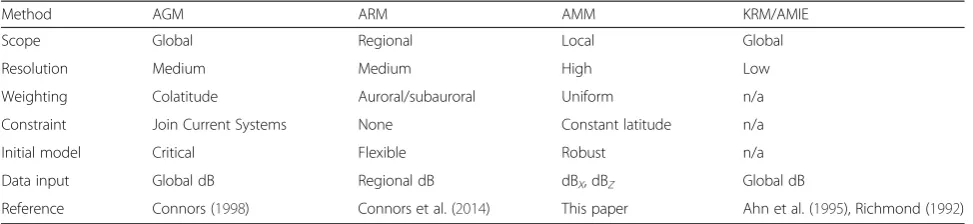
Although the basic methods of modeling and optimization are applicable generally, constraints and weighting also play a large role in data inversion, and nonuniqueness can be a special challenge (Li and Oldenburg 1996). For para-metric inversion, the role of initial parametrization or“an initial guess for parameter values”can also be important. All of these factors play a role in the functional division of AFM into global (AGM), regional (ARM), and meridian (AMM) approaches, which share a compute module but have different constraints, weighting (including not using certain components), and initial condition requirements. These approaches are summarized in Table 1.
perturbations. If only stations very near the electrojet are used, AMM can have uniform station weighting as indi-cated in the table, however (for example, in the second ex-ample below, with further discussion in the Appendix), it is also possible to judiciously apply weightings. AMM uses only the perturbations along the local magnetic north (dBX) and vertically down (dBY) directions.
To represent surface magnetic field perturbations due to near-Earth electric currents, one requires a model specifying the perturbations that would arise at the sur-face, as a function of parameters which usually can be chosen to be physical quantities, as described in the next section. Those parameters can be varied through the above recipe until an optimized match between model output and the observed fields at many points is ob-tained. The parts of the model circuit which are nearest the observing sites contribute most to the modeled per-turbations at those sites, so that the entire closed current system in space is not used. Not only are the details of the distant parts of the system the least well known but compared to smaller local current systems and inaccur-acies resulting from a simplified model, the contribu-tions from those parts are small (Friedrich et al. 2000).
Electrojet magnetic field model
In practice, the method of Kisabeth (1972, 1979) and Kisabeth and Rostoker (1977) has been used in calculating the magnetic perturbations due to model current systems. This technique has a spherical Earth, induction treated through a superconductor at depth (usually chosen as 250 km), and FAC following dipole field lines. In this simple view, an auroral electrojet may be regarded as being char-acterized by FAC flow into the ionosphere, flow within the ionosphere for some distance, and then FAC flow out of the ionosphere. The regions in which FAC intersects the ionosphere may be regarded as sheets of current without much loss of generality: in this case, the coordinates of two points must be given to specify the end points of the each sheet. Since there is one sheet of downward FAC and one of upward FAC for each electrojet, eight geometric parameters are required to specify such a system, a ninth being the total electric current (Connors 1998; Connors
and Rostoker 2002). If one sheet is north of the other and the system has large east–west extent, the resulting north–south (poloidal) ionospheric currents joining them would be primarily Pedersen currents and their ground perturbations small (Boström 1964). Associated auroral arcs would be aligned east–west, and toroidal current par-allel to them would produce most of the magnetic effect on the ground. The electric field must be known to deter-mine if a given ionospheric current is a Hall or Pedersen current, but to perform the Biot-Savart integral, it is not necessary to know the nature of the electric current, merely where it is and its strength.
The “long narrow toroidal current” case is often ap-plicable to modeling data from magnetic meridian chains and is emphasized in this article. In this case, only three parameters (two latitudinal limits and a current strength) characterize the electrojet as observed far from the FAC, whose influence is taken to be small. Of course situations arise, such as being near an auroral surge (Weimer et al. 1994), where intense FAC are near an observing station and this approximation is not valid. In this case, a largeY(eastward) component field magni-tude would be present, so that it is easy to identify and exclude such cases.
The north–south perturbation component due to an east–west aligned ionospheric current system has a max-imum in intensity directly below the center of the current (Kisabeth 1979). This is flanked by extrema of the vertical component. Application of the modeling technique described above is straightforward with such current systems. The squared deviationχ2between mea-sured ground signatures and perturbations calculated from the forward model current system is determined. The above procedure is used to vary the parameters of the model until the minimum of χ2 is obtained. Since the ground effects of the electrojets are largely due to roughly east–west aligned (nominally Hall) current flow, this simple technique allows the basic parameters of this current flow to be determined.
The perturbations observed by satellites traversing FACs associated with the poleward (region 1 or R1) and equatorward (region 2 or R2) borders of the auroral oval
Table 1Contrasting versions of automated forward modeling and global EM solvers
Method AGM ARM AMM KRM/AMIE
Scope Global Regional Local Global
Resolution Medium Medium High Low
Weighting Colatitude Auroral/subauroral Uniform n/a
Constraint Join Current Systems None Constant latitude n/a
Initial model Critical Flexible Robust n/a
Data input Global dB Regional dB dBX, dBZ Global dB
are familiar (Iijima and Potemra 1978). The ground per-turbations due to such currents are usually small and often ignored but have a characteristic disturbance pat-tern differing from that of the Hall electrojets (Kisabeth 1979). Although the perturbations from the north–south systems are small, they are not zero, while Fukushima’s (1969) theorem is often cited to suggest that they should be. There is no contradiction, since the theorem applies only to a uniformly conducting ionosphere, and that is not the case in the auroral zone. The fact that the per-turbation pattern from the R1/2 (region 1 and 2 FAC) and Pedersen ionospheric system is different from that of the Hall electrojets allows, at least in principle, the detection of the R1/2 FAC from the ground. Tamao (1986) pointed out that oblique FAC may also be detect-able from the ground, but that this effect is most pro-nounced for systems whose east–west length is short compared to their north–south extent. Here, we concen-trate on the opposite case of long electrojets. In contrast, Kawasaki and Rostoker (1979) found that the ground magnetic effects of Ps 6 perturbations, which are mostly in theYandZ components, could be well explained by eastward drifting current systems of short east–west ex-tent: this interpretation is consistent with the results of Tamao (1986). This study concentrates on cases in which there is not a largeYcomponent and does not at-tempt to determine FAC associated with electrojets. An important aspect of FAC associated with net current supply to the toroidal electrojet is that in cases where such FAC is distant, the distinction between physical current which is determined by AFM and equivalent current determined by some other methods disappears. This issue is treated below.
Having outlined how AFM can be applied to inversion of magnetic data, we now present its use in event studies where the AMM variant can be applied to inversion in single meridians.
Results
April 1, 1986 event
We will first examine an older substorm event to give an overview of the uses of magnetic inversion. Due to good auroral imaging and ground data available, this event was selected as“Event A”for the CDAW-9 campaign of substorm studies. With expansive phase onset at 18:50 UT April 1, 1986, it was presented as prototypical of the
“eye” appearance of UV manifestation of substorm expansive phases as seen from the Viking satellite by Rostoker et al. (1987). It was also discussed with focus on the use of satellite optical data to interpret substorm onsets by Murphree et al. (1991). A magnetic data set put together by Ahn et al. (1995) allowed them to study this event using the KRM method, with instantaneous conductivity based on Viking images. An inversion
method determining magnetic local time (MLT) of currents (but not their strength) from midlatitude variations per-mitted Sergeev et al. (1996) to study this event in con-junction with images from the Viking satellite. Another study (Lu et al. 1997) is based primarily on AMIE and also presents GOES results, with an emphasis on map-ping and no specific attention to the SCW total FAC. Here, we describe the event and assess the role of AFM in studying electrojets in such events. The overall situ-ation with the auroral event well developed is shown in the transformed Viking spacecraft image of Fig. 1. By this time, the “eye of the substorm” had expanded northward (Rostoker et al. 1987). The auroral currents and in par-ticular the westward electrojet flowed over the then extant Russian Kara Sea chain. The Russian observations were presented at low cadence (5 min) to CDAW-9 for analysis and obtained from the CDAW-9 CD-ROM.
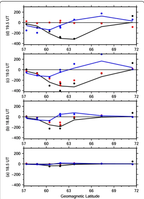
Figure 2 presents a stack plot of magnetic perturba-tions for four periods in the development of the substorm as a function of latitude. Dots represent obser-vations, and model results are shown as solid lines for the X (northward) and Z (downward) components. The Ycomponent is not used in simple electrojet modeling, and a model value is not shown. In the middle two panels, the Ycomponent follows the X component and is negative (westward). This could arise from the electro-jet being tilted toward the northwest, and this image leads to believe this could be a realistic configuration. However, in what follows, we assume the “westward electrojet” flowed due west. Allowing for tilt would give a slightly larger current than derived here. Figure 2a shows −X perturbations centered at about 61°, with +Z to the north and−Z to the south. This is the signature of a westward electrojet. In Fig. 2b, shortly after the time of onset, the electrojet is stronger and now centered at 62°. In Fig. 2c, the electrojet was centered at 64°, and the larger amplitude of perturbations indicates a
strengthened current. In the northern half of the electro-jet,Zis not large enough in the model, which may be due to structure in the electrojet not present in the model’s uniform electrojet. An enhanced current density at the poleward border would account for this and is possible to implement, but we are striving for a simplest possible model. In Fig. 2d, the perturbations are smaller but in close to the same locations, indicating little change in pos-ition in a half hour, but some weakening of current. Stack plots permit one to see that the electrojet model repre-sented the data well, but it is the simple parameters de-rived from modeling that have the most utility.
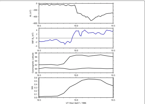
Figure 3 shows (from bottom up) the model parame-ters of cross-meridian current and electrojet borders, the interplanetary magnetic field northward component, and the standard AL index, the latter two from the OMNI database. It is clear (even from the low cadence data inverted) that substorm onset with the classic signatures of strengthening of the westward electrojet and poleward motion of the electrojet (here only the northern border)
took place at 18:45 and was well underway at 18:50, the latter being the time found in other studies. However, the AL (1-min) index did not drop until 18:59 UT. Since this is very shortly after northward turning of the IMF, a causal relation could be inferred if AL was used as the timing indicator for this substorm. In fact, onset took place before the northward turning in the (propagated) OMNI data. As pointed out by Rostoker (1972) and reiter-ated by Connors (2012), the AL index must be used with care in individual events. However, we have succeeded showing that the use of simple physical parameters, even with low cadence, allows good timing and gives current strength and latitudes that could be used for mapping.
We now proceed to describe another defunct magnet-ometer chain but one allowing high-quality inversions useful in the THEMIS era.
Polaris chain inversion
The Polaris geophysical project emplaced geophysical in-struments in several locations in Canada (Bastow et al. 2015) including the east shore of Hudson Bay and southward, as the Hudson Bay Lithospheric Experiment (HuBLE). The instruments included magnetometers pro-ducing high cadence data, available with gaps during the first years (2007–2012) of the THEMIS (Angelopoulos 2008) mission. The Polaris East Hudson Bay array, for which a map is given in Fig. 4, may be seen as the prede-cessor of the new AUTUMNX array (Connors et al. 2015) and had more stations in its meridian chain aligned with the east coast of Hudson Bay. As such, its dense network of stations is suitable for demonstrating inversion, especially when combined with other nearby stations such as those of MACCS (Hughes and Engeb-retson 1997) and NRCan Canadian federal government observatories.
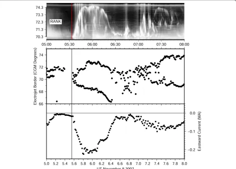
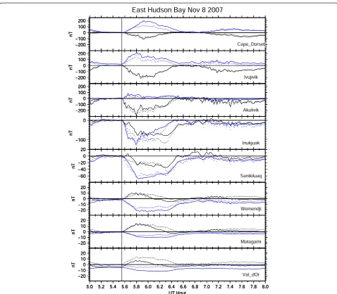
We did inversion using the stations listed in Table 2, using as reference a quiet day on November 6, 2007, whose data were smoothed with a 1-h boxcar filter. Figure 5 shows inversion results for a simple westward electrojet for a substorm with onset time 5:33 UT on November 8, 2007. The bottom panel shows eastward current, plotted as negative values to resemble the AL index, and this attained a magnitude of about 0.2 MA. The electrojet borders widened from the time of onset both toward the north and the south by about 3°. At the end of the current intensification, the poleward border retreated equatorward, and a period of unsettled activity followed. Although the date was after the launch of the THEMIS constellation, no spacecraft were in interesting locations ex-cept GOES 10, GOES East at the time, which showed a small dipolarization signature (data not shown). THEMIS ground instrumentation at Rankin Inlet (RANK), on the west shore of Hudson Bay at CGM (Gustafsson et al. 1992) latitude approximately 72.3 °, did optically detect the
substorm (the imager south of Rankin, Gillam, had cloudy weather). The imager at RANK detected a brightening near the southern horizon at the time of magnetic onset (5:33 UT) and rapidly poleward moving auroras, approaching the northern horizon at approximately 6 UT, and subsequently retreating equatorward to be followed by auroral activity. We cannot tell from the optical data if there was equator-ward expansion of the auroras, but the overall poleequator-ward ex-pansion was to about the same width as the magnetically inferred electrojet boundaries. The overall shape in latitude-time space was similar during the expansive/ early recovery phase lasting from 5:33 UT to nearly 6:30 UT. Reference to Fig. 1, the“eye” of the substorm, would lead one to expect some differences over the ap-proximately 2 h of local time separating Polaris from RANK, but in general a simple electrojet model shows the same behavior as that inferred from a keogram, with the advantage that the electrojet borders and current are nu-meric values able to be used for other purposes.
Within the array itself, one can get an idea of the util-ity of the simple model by comparing input data to the results from the model’s parameters. Figure 6 shows a
stack plot ofX(black) and Z(blue) perturbations as ob-servations (solid) and model results (dots). In general, there is a very good reproduction of the input data through the use of only the three simple parameters of north and south electrojet borders and total current. The stations with large signal seem to have the best fit, which may suggest that adjusting the weighting of input data could improve the model. We present a detailed statistical analysis of the fitting in the Appendix. We do not know the position of field-aligned current for the SCW of this event (although it could to some extent be inferred from subauroral perturbations). We discuss an event in which it is known from external data in the next section. There is also a period before the substorm onset when perturbations were weak and the model did not converge. Growth phase phenomenology remains of great interest and we have done a more specific study of this substorm phase in a section below for which the perturbations were more pronounced, and optical data from the same meridian were available.
The basic result here is that a chain with good latitu-dinal spacing can produce useful inversions of electrojet
activity. The similar AUTUMNX chain can produce similar results (Connors et al. 2015).
Cross meridian and 1-D equivalent currents
The practice of using a three-dimensional current sys-tem representing a physical set of currents, yet placing FAC far away when inverting data from a meridian chain, allows a parallel to be made between AMM and methods that determine an equivalent current, such as spherical elementary current systems or SECS (Amm and Viljanen 1999). When FAC systems are placed far enough away to have minimal effect in the model, the ionospheric current system crossing the meridian is equivalent to the divergence-free elementary system which flows in a toroidal direction in the SECS method. We can thus reconcile the view that parameters of
three-dimensional physical current systems may be de-termined from the ground, as Connors et al. (2014) demonstrated by comparison with AMPERE space-based data (Anderson et al. 2014), and the stricter view that they cannot. For meridian chain inversion with distant FAC, the AFM method should be essentially determining the divergence-free part of the current system and get the same result as SECS used in 1-D form over a merid-ian chain. We proceed to demonstrate empirically that this is the case. Further, using AMPERE data, we show that the cross-meridian current determined by AMM is the same as that in the net FAC of the SCW, which is added on to pre-existing R1 currents.
By browsing the maps of AMPERE-determined radial current (essentially FAC at auroral latitudes), showing landmasses, available at http://ampere.jhuapl.edu/rBrowse/ index.html, we determined that a substorm on January 15, 2010, with onset time 20:37 UT, bracketed Fennoscandia in a way that should have produced a substorm westward electrojet over the IMAGE array. An electrojet inversion was performed using an automated version of SECS avail-able on the IMAGE (Tanskanen 2009) FMI website (http:// www.ava.fmi.fi/MIRACLE/iono_1D.php) with baseline rela-tive to a quiet period earlier in the UT day. An AMM in-version was performed using the same data downloaded to a local computer. The eastward current in the event as de-termined by the two techniques is shown in Fig. 7 in the bottom panel, as before, negative values indicating that the current was actually westward. The two results agree to within about 10 %. The SECS result also produced an east-ward current during the early stage, which although not shown would reduce the difference. After the minimum, the SECS result was slightly smaller in magnitude than the AFM result. As the SECS eastward current was not large at this time, this does not explain the difference then.
The middle panel of Fig. 7 shows the electrojet bor-ders. These appeared poorly determined near the time of onset; but when the current became large enough, these followed a pattern similar to that in a color density plot (not shown) based on the online SECS technique. The top panel shows the IMF during the period of interest, which appears to indicate that the event was largely caused by negativeBZin the IMF, in the well-understood
manner (Baumjohann 1986).
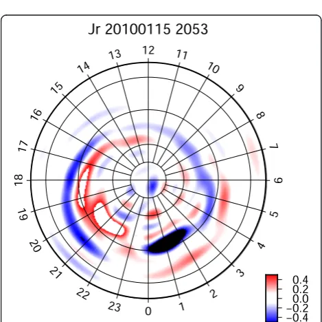
In order to compare the cross-meridian current, which AMM takes as a physical current modeled by the Biot-Savart integral, and SECS as an equivalent current, to the likely physical current, the integration technique for AMPERE data developed by Connors et al. (2014) was applied to AMPERE current densities. Figure 8 shows a snapshot of these current densities at 20:53 UT, a time marked in Fig. 7 by a vertical bar near the time of max-imum (westward) current flow. The pattern shown was typical of that during the substorm: downward current
Fig. 5Eastward Current across the Polaris chain on November 8, 2007 from 5 UT to 8 UT (bottom). Electrojet borders in magnetic coordinates (middle). THEMIS imager keogram from Rankin Inlet (top). Time of onset is marked by avertical line
Table 2Site names and locations for inversion results
Place Code Geomagnetic
longitude
Geomagnetic latitude
Magnetic longitude
Magnetic latitude
Inverse weight
Notes
Cape Dorset
CDRT 283.4 64.2 1.9 73.4 1 MACCS station
Ivujivik HUB7 282.09 62.42 359.61 71.86 1 Denoted Inujivik in data
files
Akulivik HUB8 281.81 60.81 358.97 70.37 1 AUTUMNX AKUL
Inukjuak HUB9 281.88 58.45 358.86 68.15 1 AUTUMNX INUK
Sanikiluaq SNK 280.8 56.6 357.1 66.5 1 NRCan observatory
Wemendji WEMQ 282.03 53.05 358.69 62.99 0.3
Matagami HUB6 282.36 49.76 358.94 59.79 0.3
Val d’Or VLDR 282.22 48.10 358.61 58.20 1 (X) AUTUMNX VLDR
0.3 (Z)
in the morning/midnight sector and upward current in the evening sector clearly represent the FAC of a SCW, much as shown by Connors et al. (2014). There is more than one upward current region in the evening sector: similarly, at earlier times, there had been more than one downward current region in the morning sector. Space does not permit more detailed description of FAC pat-terns at all stages of the substorm, but these may be ex-amined at http://ampere.jhuapl.edu/rBrowse/index.html. We note that in the evening sector, there is a clear R1/2 pattern corresponding to the pattern found in an aver-aged sense by Iijima and Potemra (1978). This is less clear in the morning sector but at other stages of devel-opment was more in evidence. We proceed here to study the currents in an integrated sense.
Throughout this event, the IMAGE chain in Fenno-scandia was located 2300 MLT, and this was near the central meridian of the substorm, being located between the clearly separated downward and upward FAC re-gions shown in Fig. 8. During the event, FAC exceeding the threshold value of 1 μA/m2occurred only between 60 ° and 80 ° geomagnetic latitude. FAC could, however, extend as far as 0900 MLT in the morning sector or 1500 MLT in the afternoon sector. From 2300 MLT to these limits, and using the latitude limits mentioned, large regions were outlined that were used as integration boxes with gridded data in the manner described by Connors et al. (2014). Integrating in the morning sector, a downward current is in R1 and an upward current in R2 south of it. In the evening sector, this pattern is
reversed. It is known that large poloidal currents can flow and close from R1 to R2 or vice versa, with little ground effect due to the solenoidal nature of the cur-rents. If the R1/R2 closure is not balanced, then toroidal current flow is expected, crossing the near-midnight central meridian of the SCW in the case of substorms.
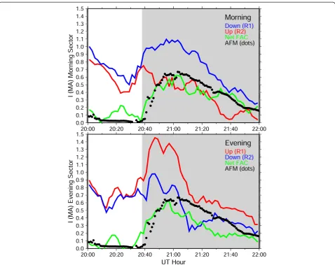
We calculated cross-meridian current independently in two ways. The difference of R1/R2 integrated currents from AMPERE data, with the assumption that current missing in the morning must have flowed toward the evening, gives the net current across the meridian. AMM based on the IMAGE magnetometer data should determine the same current independently. The results of AMPERE integration and of AMM are shown in Fig. 9. In each of the morning and evening sectors, we integrated the R1 and R2 currents. The downward and upward current totals in the morning and evening integration boxes are shown with blue and red lines, respectively. Their difference is shown with a green line. In the morning sector, the R1 current is downward, as indicated by a red line, and the R2 current is upward and indicated with a blue line. In the evening sector, the associ-ation of R1 and R2 with color is reversed.
If R1 and R2 currents were the same, then they must have closed in nearly poloidal fashion (that is, locally) with no cross-meridian current. This was the case before substorm onset, with variations in the green line more likely associated with uncertainty in the integrated current magnitudes than with any physical effect (the green line represents the difference of two relatively large numbers while it is small, so that uncertainties are more apparent). The results of AMM integration based on IMAGE magnetometer data are indicated by black dots. The green line in the morning sector (top) panel closely follows the AMM results. This is also the case in the evening sector. We conclude that the difference of R1 and R2 integrated currents in the morning sector was the cross-meridian current and matched that calcu-lated from AMM; in the evening sector, this difference also matched AMM. In the morning sector, the down-ward current (blue), which is in R1, increased, while in the evening sector the upward current (red), also in R1, increased. These currents flowed across the meridian and caused the ground magnetic perturbations in the IMAGE meridian, as evidenced by the AMM results showing the same current magnitude. Connors et al. (2014) concluded that the bulk of the substorm current flowed in R1: here, this result is verified.
In the pre-substorm time (white region in Fig. 9), R1 and R2 integrated currents as determined by AMPERE were between 0.5 and 1.0 MA but closely balanced, leav-ing little cross-midnight current. Durleav-ing this period, AFM indicated a low cross-meridian current. At onset time, the downward current in the morning sector and the upward current in the evening sector both rose.
Fig. 7Cross-meridian physical current from AFM (black dots) and equivalent current digitized every 0.1 h and extremal points (red line) for the IMAGE array on January 15, 2010 (bottom). Electrojet boundaries from AFM (middle panel). IMF GSE magnetic field (top panel)
Their difference closely tracked the AFM current (which in turn was very close to the SECS equivalent current). As found by Connors et al. (2014), the morning sector FAC current more closely followed the AFM current than did the evening sector FAC current. However, here, the evening sector upward current did not persist as in that case. Quantitatively, an increase of up to 0.6 MA in morning sector downward FAC was measured along with a very similar increase in evening sector upward FAC. These give rise to FAC differences very closely tracking the cross-meridian true (AMM) or equivalent (SECS) currents in the ionosphere.
It was the aim of this subsection to investigate to what degree AFM agreed with SECS equivalent currents in a substorm event, and in turn to verify that the cross-meridian current indicated by those methods corre-sponded AMPERE’s determination of net FAC difference between morning and evening sectors. Much as in
Connors et al. (2014), we find a consistent picture be-tween the parameters derived from independent ground magnetometer and AMPERE in situ data. This verifies that it is possible to quantify the simple SCW model of McPherron et al. (1973) in a physically meaningful way, and this case based only on cross-meridian current that forms part of the SCW.
Growth phase currents
A final example pushes AMM to its limits. The previous examples succeeded during substorm expansion, with magnetic perturbations in the hundreds of nT and cur-rents of several hundred kA, but did not converge well based on the weak currents before onset. Growth phase typically features such much smaller perturbations and in turn, currents. Figure 10 shows magnetic variations on February 22, 1997, using smoothed data from February 19, 1997 as a quiet day reference. Due to the fortuitous
occurrence of a good quiet day nearby in time, small vari-ations due to local currents are detected. A small expan-sive phase onset took place at 3.77 UT (03:46 UT), as manifested by the decrease in theXcomponent at several stations at that time and the corresponding changes in the Zcomponent. We did not model that expansive phase but rather the growth phase preceding it. We used data from the CANOPUS Churchill line, the predecessor array to CARISMA (Mann et al. 2008). The event took place in the evening sector, where the growth phase was mani-fested mainly by an eastward electrojet.
OMNI data (see Fig. 11) had a southward IMF aver-aging about−4 nT during the period 1:00–3:30 UT, with a brief northward turning at 2:00 UT. Thus, the normal growth phase pattern of expansion of the auroral oval was taking place. Positive X component perturbations moved to lower latitudes as time progressed, moving from ESKI to GILL, indicating equatorward motion of the evening sector auroral oval, as seen in Fig. 10. Z component changes also took place, but it is difficult
from a stack plot to decipher exactly what combination of electrojet movement and change of strength of east-ward current occurred. We note from the dots in Fig. 10 that a generally good match to data was obtained with a simple electrojet model.
Figure 11 presents the output parameters of that model during the growth phase, overplotted on the out-put of a meridian scanning photometer for 557.7-nm electron precipitation aurora at Gillam (station GILL). At the top is the OMNI IMF Bz. Examining the AMM output first, we note that the eastward current across the meridian was decreasing until time 3.2 UT (3:11). The equatorward boundary of the electrojet moved steadily southward throughout the period, however ac-celerated when the IMF turned more southward. At this time, the aurora also brightened considerably. The pole-ward boundary of the electrojet also moved steadily equatorward. This motion took place even as the current weakened, and the current weakening appeared to have no relation to auroral brightness. After 3.2 UT, the
current started to increase, without much change in aur-oral brightness. The overall width of the electrojet nar-rowed, with the current near 0.05 MA after 3.5 (3:30) UT. Finally, immediately before onset, the current rose dramatically, nearly doubling. After this point, the signal was dominated by intrusion of the westward electrojet of the expansive phase, with its negative perturbations in X, and was not studied.
An important aspect of Fig. 11 is that it again shows AFM results compared to an independent dataset. While the poleward boundary of the evening sector electrojet is defined optically by electron precipitation causing aurora, the equatorward boundary is dark and only indicated by AMM. The results suggest a narrowing of the electrojet and a rise in the current it carries, as immediate precur-sors of onset.
Discussion
We have described how the Levenberg-Marquardt algo-rithm, coupled with a magnetic field model, may be ap-plied to ground magnetic data in general as a procedure
we call AFM and then used it for meridian chains of sta-tions in the form we denote AMM. AMM can yield insight into the gross physical parameters of electrojets which change during substorms. Despite using only the two electrojet borders and the cross-meridian current, good reproduction of the input data is demonstrated, so that we can conclude that the simple modeling parame-ters represent a large part of the variation in physical pa-rameters during the events studied.
We showed the technique applied to a previously extensively studied substorm, and how even with low time resolution, inversion results can give a clearer pic-ture of timing than can the AL index. We provided infor-mation about the Polaris predecessor of the AUTUMNX network in Québec (eastern North America) and an ex-ample of inversion using data from that chain. We empha-sized that comparison of output model results to input is essential in knowing to what degree a simple model repre-sents electrojet activity. We then compared the results of AMM as applied to a meridian for which both the SECS reduction technique and AMPERE integrations
could also determine cross-meridian current. We found that all three techniques gave similar results. The phys-ical picture provided by AMPERE’s measurement of FAC reinforced the concept that AFM can invert ground data into a three-dimensional framework re-sembling the original SCW. We noted that in any case, far from the FAC normally present in the AFM model, its cross-meridian current is divergence-free and thus directly comparable to the equivalent current in a 1-D SECS application. Finally, we found that AMM used on very carefully baselined growth phase data could extract information about the eastward electrojet that was, at least in the motion of the poleward border, verifiable from an independent optical dataset.
Conclusion
The AFM technique in its AMM form has been shown here to allow a simple and efficient representation of magnetic meridian data. Its output parameters have been shown to correspond to physical parameters of the elec-trojet system by comparison to other indicators. AFM is extensible as has been shown by use of ARM by Con-nors et al. (2014) and less successfully on a global scale (AGM) by Connors (1998) and should be helpful in our quest to understand substorm electrodynamics.
Appendix
Statistics of automated meridian modeling data representation
The intent of AMM is to represent observations of per-turbation magnetic fields in a meridian with a simple representation of the electrojet. Figure 5 presented the parameters of a uniform electrojet current between two latitudinal boundaries which AFM found to optimally represent the perturbations measured by the Polaris array on November 8, 2007. The agreement of the model output with measured data was shown in Fig. 6. Here, we quantify the degree to which the simple model rep-resented the data using standard statistical methods (see, e.g., Press et al. 1992).
In all variants of AFM, the objective function is based on weighted perturbation data. The aim of weighting is to allow all relevant information to enter the solution without bias such as that from large data values (Li and Oldenburg 1996). The choice of weights is somewhat subjective and we prefer not to vary them from one run to another, but this could be done. This point is not fur-ther considered here. Instead, we examine to what de-gree the simple model did represent the unweighted original data, a good representation being essential to the argument that the parameters derived are physically meaningful.
In the ideal case, values calculated from the deduced model would exactly match the input data at all stations.
At any given station, a plot of model value against ob-served value would give points lying on a straight line of slope 1 and zero intercept. The Pearson r coefficient would be 1, and with no difference between the model output and the data, the standard deviation of their dif-ference would be zero. We proceed first to give formulas for calculation of these parameters and then present results at representative stations in graphical and tabular form.
The optimal fit line from Gaussian regression with y the model output and x the data input value is y=a+ bx, withathe intercept of the fit andbits slope. If there areNinput pointsxiof original data represented by
cor-responding model output points yi, where i= 1…N, we
Δ . There are two commonly used indicators of
goodness of fit, each involving the average values of the input data x¼Sx=N and model output y¼Sx=N. The Pearson r coefficient, r¼
X
takes on values between 0 and 1 for degrees of positive correlation between none and perfect matching (its pos-sible negative values do not concern us here). Finally,
the standard deviation σ¼ ffiffiffiffiffiffiffiffiffiffiffiffiffiffiffiffiffiffiffiffiffiffiffiffiffiffiffiX i
xi−y xð Þi
ð Þ
r
gives an idea
of the scatter of points around the regression line where y(xi) =a+bxi. We have selected three stations for a
de-tailed examination of these metrics. As seen in Fig. 6, subauroral station Matagami showed a positive BX and
negative BZas expected for a subauroral location inside
the SCW. Inferred to be south of the westward electrojet center, Inukjuak had a negative BX perturbation and also
negativeBZ. With negativeBXand near-zeroBZ,Akulivik was near the electrojet center during the active period. Al-though variations in the goodness of match of model to data took place during the event, we considered the entire period shown. The Val d’Or station appeared to have off-sets left over from baselining so was not chosen for dis-cussion: the auroral zone stations are typical of the other more northerly stations.
quantified as the standard deviation listed in Table 3’s last column.
In general, with small intercepts and slopes which are close to one, in all cases, there is a good match between model output and the original data. Pearson r coeffi-cients in all cases above 0.85 indicate a very good repre-sentation. The scatter is a small fraction of the maximal perturbations observed at each station. All of these
results are consistent with the closeness of the model and data traces in Fig. 6. Certain aspects of the modeling at each station bear further discussion, however.
At Matagami, the slopes of both BX and BZ
compo-nents are smaller than implied by the electrojet model, despite a fairly good overall fit. We may take this to imply different causation and would suspect a large ef-fect of field-aligned currents, which we nominally do not −10
0 10 20
Model X
−10 0 10 20 Matagami X
−10 0 10 20
Model Z
−10 0 10 20 Matagami Z −150
−100 −50 0 50 100
Model X
−150 −100 −50 0 50 100 Inukjuak X
−150 −100 −50 0 50 100
Model Z
−150 −100 −50 0 50 100 Inukjuak Z
−300 −200 −100 0 100
Model X
−300 −200 −100 0 100 Akulivik X
−300 −200 −100 0 100
Model Z
−300 −200 −100 0 100 Akulivik Z
Fig. 12Scatter plots of the model output along theXandZaxes
Table 3Statistics of model representation of data at three Polaris stations
Station Component a(intercept) (nT) b(slope) (no units) Pearsonr Scatterσ(nT)
Matagami X 2.39575 0.814831 0.85114 2.03111
Matagami Z 0.4521 0.667355 0.929067 0.763273
Inukjuak X −2.18033 1.31782 0.968573 9.00434
Inukjuak Z −4.26947 1.09909 0.945252 11.0123
Akulivik X −10.7291 1.10217 0.975994 15.4632
include in AMM by making them relatively far from the meridian modeled. Field-aligned dominance at midlati-tude was already present in the original SCW model (McPherron et al. 1973) and supported also by studies by Sun et al. (1984). This consideration may suggest fur-ther examination of inclusion of midlatitude stations when doing AMM inversions. At Inukjuak, the slope of re-sponse for bothBXandBZwas larger than one. We
attri-bute this to being near the southern border of the electrojet, where small inaccuracies in its exact location could lead to large changes in the modeled perturbations. The scatter is of order 10 nT in each component, of order 10 % of the perturbation. At Akulivik, inferred from small
values of BZ to be near the center of the electrojet, the
slope forBXis close to one, likely reflecting a lack of
sensi-tivity to small positional changes in this location of its maximal amplitude. On the other hand, the opposite con-sideration should apply for BZ, yet its slope is considerably lower. At this time, we do not have a good explanation for this. Here, the scatter was larger than at Inukjuak, which in theXcomponent may be explained partly by a possible anomalous ground response which we have inferred by examining magnetotelluric data (not shown).
In summary, quantitative analysis shows a good de-gree of reproduction of data from near the electrojet by the limited number of parameters used in AMM. We 0
20 40 60 80 100
−10 0 10
Matagami X
0 20 40 60 80 100
−10 0 10
Matagami Z 0
10 20
−40 −20 0 20 40 Inukjuak X
0 10 20
−40 −20 0 20 40 Inukjuak Z
0 10 20
−40 −20 0 20 40 Akulivik X
0 10 20
−40 −20 0 20 40 Akulivik Z
thus attribute meaning to those parameters: there are often well-defined borders to the electrojet, and the current across a meridian is well inferred from AMM inversion. Possibly, with very dense meridian chains, one could deduce information about structure in electrojets.
Abbreviations
AFM:automated forward modeling; AGM: automated global modeling; AMM: automated meridian modeling; ARM: automated regional modeling; AMIE: assimilative modeling of ionospheric electrodynamics; AMPERE: Active Magnetosphere and Planetary Electrodynamics Response Experiment; BX: magnetic field along the local magnetic north (X) direction; BZ: magnetic field component vertically downward,or in IMF, northward component; CGM: corrected geomagnetic (coordinates); dB: magnetic perturbation, here due to auroral current systems; FAC: field-aligned current; IMF: interplanetary magnetic field; KRM: Kamide-Richmond-Matsushita (modeling method); R1: region 1 (poleward) FAC in Iijima and Potemra (1978) terminology; R1/ 2: region 1/region 2; R2: region 2 (equatorward) FAC in Iijima and Potemra (1978) terminology; SECS: spherical elementary current systems (modeling method); SCW: substorm current wedge.
Competing interests
The authors declare that they have no competing interests.
Authors’contributions
MC developed and applied AFM techniques. The original concept of AFM is due to GR. Both authors read and approved the final manuscript.
Authors’information
MC is a Professor of Space Science and Physics at Athabasca University and PI of the Athabasca University Observatories and AUTUMNX. He holds a Ph.D. in Physics from the University of Alberta. GR is an Emeritus Professor of Space Physics at the University of Alberta.
Acknowledgements
This work was supported by NSERC and in part by the Canada Research Chairs program. The CANOPUS chain was operated by the Canadian Space Agency. We thank Andrei Kotikov for supplying Russian data used for the April 1, 1986 study to the CDAW-9 project. Polaris data were obtained from NRCan. We thank the institutes who maintain the IMAGE magnetometer array and Eric Donovan and Emma Spanswick of the University of Calgary for THEMIS keograms and calibrations, from cameras supported by the Canadian Space Agency. We also thank the AMPERE team and the AMPERE Science Center for providing the iridium-derived data products and Haje Korth for special effort in that regard. Cape Dorset magnetic data was supplied by Erik Steinmetz and Mark Engetbretson of Augsburg College, via CDAWeb.
Author details
1Athabasca University Observatories, 1 University Drive, Athabasca, AB T9S 3A3, Canada.2Department of Physics, University of Alberta, Edmonton, AB T6G 2E1, Canada.
Received: 29 April 2015 Accepted: 27 August 2015
References
Ahn B-H, Kamide Y, Kroehl HW, Candidi M, Murphree JS (1995) Substorm changes of the electrodynamic quantities in the polar ionosphere: CDAW 9. J Geophys Res 100:23845–23856
Amm O, Viljanen A (1999) Ionospheric disturbance magnetic field continuation from the ground to the ionosphere using spherical elementary current systems. Earth Planets Space 51:431–440
Anderson BJ, Korth H, Waters CL, Green DL, Merkin VG, Barnes RJ, Dyrud LP (2014) Development of large-scale Birkeland currents determined from the active magnetosphere and planetary electrodynamics response experiment. Geophys Res Lett 41:3017–3025. doi:10.1002/2014GL059941
Angelopoulos V (2008) The THEMIS mission. Space Sci Rev 141:5–34. doi:10.1007/ s11214-008-9336-1
Bastow ID, Eaton DW, Kendall J-M, Helffrich G, Snyder DB, Thompson DA, Wookey J, Darbyshire FA, Pawlak AE (2015) The Hudson Bay Lithospheric Experiment (HuBLE): insights into Precambrian plate tectonics and the development of mantle keels. Geol Soc Lond, Spec Publ 389:41–67 Baumjohann W (1986) Some recent progress in substorm studies. J Geomag
Geoelectr 38:633–651
Boström R (1964) A model of the auroral electrojets. J Geophys Res 69:4983–4999 Connors M (1998) Auroral current systems studied using automated forward
modeling, Ph.D. Thesis, Department of Physics, University of Alberta, Edmonton, Canada
Connors M (2012) Comment on“Substorm growth and expansion onset as observed with ideal ground spacecraft THEMIS coverage”by V. Sergeev et al. J Geophys Res 117:2. doi:10.1029/2011JA017254
Connors M, Rostoker G (2002) A substorm sequence studied with automated forward modeling. In: Winglee R (ed) Sixth international conference on substorms. University of Washington Press, Seattle WA
Connors M, McPherron RL, Anderson B, Korth H, Russell CT, Chu X (2014) Electric currents of a substorm current wedge on 24 February 2010. Geophys Res Lett 41:4449–4455. doi:10.1002/2014GL060604
Connors M, Schofield I, Reiter K, Chi PJ, Russell CT, Rowe K (2015) The AUTUMNX magnetometer meridian chain in Québec, Canada. Earth Planets Space, this issue
Friedrich E, Rostoker G, Connors M, McPherron RL (2000) Comment on“A Note on Current Closure”by V. Vasyliunas. J Geophys Res 105:27841–27842 Fukushima N (1969) Equivalence in ground geomagnetic effect of
Chapman-Vestine’s and Birkeland-Alfvén’s electric current-systems for polar magnetic storms. Rep Ionos Space Res Japan 23:219–227
Gustafsson G, Papitashvili NE, Papitashvili VO (1992) A revised corrected geomagnetic coordinate system for epochs 1985 and 1990. J Atmos Terr Phys 54:1609–1631
Hughes WJ, Engebretson MJ (1997) MACCS: magnetometer array for cusp and cleft studies. In: Lockwood M, Wild MN, Opgenoorth HJ (eds) Satellite– ground based coordination sourcebook, ESA-SP-1198. European Space Agency, Noordwijk
Iijima T, Potemra TA (1978) Large-scale characteristics of field-aligned currents associated with substorms. J Geophys Res 83:599–615
Kamide Y, Baumjohann W (1993) Magnetosphere-ionosphere coupling. Springer, Berlin
Kawasaki K, Rostoker G (1979) Perturbation magnetic fields and current systems associated with eastward drifting auroral structures. J Geophys Res 84:1464–1480
Kisabeth JL (1972) The dynamical development of the polar electrojets. Ph.D. thesis, University of Alberta, Edmonton, Alberta, Canada
Kisabeth JL (1979) On calculating magnetic and vector potential fields due to large-scale magnetospheric current systems and induced currents in an infinitely conducting earth. In: Olson WP (ed) Quantitative modeling of magnetospheric processes. American Geophysical Union, Washington DC Kisabeth JL, Rostoker G (1977) Modeling of the three-dimensional current
systems associated with magnetospheric substorms. Geophys J R Astron Soc 49:655–683
Lampton M (1997) Damping-undamping strategies for the Levenberg-Marquardt nonlinear least squares method. Comput Phys 11:110–115
Li Y, Oldenburg DW (1996) 3-D inversion of magnetic data. Geophysics 61:394–408
Lu G, Siscoe GL, Richmond AD, Pulkkinen TI, Tsyganenko NA, Singer HJ, Emery BA (1997) Mapping of the ionospheric field-aligned currents to the equatorial magnetosphere. J Geophys Res 102:14467–14476
Lühr H, Geisler H, Schlegel K (1994) Current density models of the eastward electrojet derived from ground based magnetic field and radar measurements. J Atmos Terr Phys 56:81–91
Mann IR, Milling DK, Rae IJ, Ozeke LG, Kale A, Kale ZC, Murphy KR, Parent A, Usanova M, Pahud DM, Lee E-A, Amalraj V, Wallis DD, Angelopoulos V, Glassmeier K-H, Russell CT, Auster HU, Singer HJ (2008) The upgraded CARISMA magnetometer array in the THEMIS era. Space Sci Rev 141:413451. doi:10.1007/s11214-008-9457-6
McPherron RL, Russell CT, Aubry MP (1973) Satellite studies of magnetospheric substorms on August 15, 1968, 9. Phenomenological model for substorms. J Geophys Res 78:3131–3149
Popov VA, Papitashvili VO, Watermann JF (2001) Modeling of equivalent ionospheric currents from meridian magnetometer chain data. Earth Planets Space 53:129–137
Press WH, Teukolsky SA, Vetterling WT, Flannery BP (1992) Numerical recipes in C, 2nd edn. Cambridge University Press, Cambridge
Richmond AD (1992) Assimilative mapping of ionospheric electrodynamics. Adv Space Res 12:59–68
Ridley AJ, de Zeeuw DL, Gombosi TI, Powell KG (2001) Using steady state MHD results to predict the global state of the magnetosphere-ionosphere system. J Geophys Res 106:30067–30076
Ridley AJ, Hansen KC, Tóth G, De Zeeuw DL, Gombosi TI, Powell KG (2002) University of Michigan MHD results of the Geospace Global Circulation Model metrics challenge. J Geophys Res 107:1290–1309. doi:10.1029/ 2001JA000253
Rostoker G (1972) Geomagnetic Indices. Rev. Geophys. Space Phys. 10:935–950. Rostoker G, Vallance-Jones A, Gattinger RL, Anger CD, Murphree JS (1987) The
development of the substorm expansive phase: the“Eye”of the substorm. Geophys Res Lett 14:399–402
Sergeev VA, Vagina LI, Elphinstone RD, Murphree JS, Hearn DJ, Cogger LL, Johnson ML (1996) Comparison of UV optical signatures with the substorm current wedge as predicted by an inversion algorithm. J Geophys Res 101:2615–2627
Sun W, Ahn B-H, Akasofu S-I, Kamide Y (1984) A comparison of the observed mid-latitude magnetic disturbance fields with those reproduced from the high-latitude modeling current system. J Geophys Res 89:10881–10889 Tamao T (1986) Direct contribution of oblique field-aligned currents to ground
magnetic fields. J Geophys Res 91:183–189
Tanskanen EI (2009) A comprehensive high-throughput analysis of substorms observed by IMAGE magnetometer network: years 1993–2003 examined. J Geophys Res 114, A05204. doi:10.1029/2008JA013682
Untiedt J, Baumjohann W (1993) Studies of polar current systems using the IMS Scandinavian magnetometer array. Space Sci Rev 63:245–390
Weimer DR, Craven JD, Frank LA, Hanson WB, Maynard NC, Hoffman RA, Slavin JA (1994) Satellite measurements through the center of a substorm surge. J Geophys Res 99:23639–23649
Submit your manuscript to a
journal and benefi t from:
7Convenient online submission
7Rigorous peer review
7Immediate publication on acceptance
7Open access: articles freely available online
7High visibility within the fi eld
7Retaining the copyright to your article