Earth Planets Space,65, 911–916, 2013
An error analysis on nature and radar system noises in deriving the phase and
group velocities of vertical propagation waves
C. C. Hsiao1, J. Y. Liu1,2,3, and Y. H. Wang1
1National Space Organization, Hsin-Chu, Taiwan
2Institute of Space Science, National Central University, Chung-Li, Taiwan
3Center for Space and Remote Sensing Research, National Central University, Chung-Li, Taiwan
(Received October 6, 2007; Revised January 11, 2013; Accepted January 17, 2013; Online published September 17, 2013)
A Fourier analysis method has been employed deriving both the phase and group velocities of the atmospheric and ionospheric waves observed by various radar instruments. In this paper, a simulation is conducted to estimate errors of the two velocities resulted from the noises of natural background and radar system. The two noises with various amplification factors are placed into both synthetic data and observations of the MU (Middle- and Upper-atmosphere) radar for further investigations and validations. It is found that the errors of the phase and group velocities caused by the system noise are approximately constants, while those by the natural background noise are generally proportional to the amplification factors. The results confirm that the method can sustain the influences from natural background and system noises.
Key words:Ionosphere, radar, error analysis, wave propagation.
1.
Introduction
Various sounding techniques ranging from VLF to UHF bands are employed to observe the ionospheric waves (Davies, 1990; Hunsucker, 1991). A Fourier analysis method has been adapted deriving the phase and group ve-locities of atmospheric and/or ionospheric waves in data of the Doppler velocity by the Chung-Li very high frequency (VHF) radar (Kuo et al., 1993), virtual height (Liuet al., 1998; Leeet al., 2002), true height by ionosondes (Altadill
et al., 2001), and echo-power by the Middle- and Upper-atmosphere (MU) radar (Liu et al., 2007). Most of the studies simply adapted this method focus on calculating the two velocities and finding the associated mechanisms of the waves. However, noises of the nature background (the at-mosphere and/or ionosphere) and of the sounding systems contributing to the data could easily affect the accuracy in deriving the phase and group velocities.
On the other hand, scientists examined the electron den-sity perturbations in incoherent scatter measurements with the MU radar (Fukaoet al., 1993; Oliveret al., 1994, 1995, 1997). These papers report the electron density perturba-tions showing downward phase propagation and parameters of the observed perturbations obey the dispersion relation of atmospheric gravity waves.
In this paper, based on the characteristic of incoherent scattering observations of the MU radar, a synthetic data is generated to investigate errors in the wave propagation by using the Fourier analysis. Simulations with various ampli-fication factors of the natural background and/or sounding
Copyright cThe Society of Geomagnetism and Earth, Planetary and Space Sci-ences (SGEPSS); The Seismological Society of Japan; The Volcanological Society of Japan; The Geodetic Society of Japan; The Japanese Society for Planetary Sci-ences; TERRAPUB.
doi:10.5047/eps.2013.01.004
system noises smearing both the synthetic wave packet and the observation are used to estimate the associated errors in the phase and group velocities.
2.
Simulation
A simulation is developed to estimate the errors response to the natural background and/or sounding system noises and validate the phase and group velocities of the atmo-spheric gravity waves in the incoherent scattering echo-power observation by the MU radar reported by Liuet al.
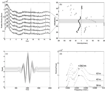
(2007). Figure 1 shows the temporal variations of the MU radar echo-power from 384 to 411 km height during 0000– 1600 local time (LT) of 17 June 2001, and the associated phase and group velocities variance at each altitude. Fig-ure 1(b) displays that the group (phase) velocity is in an up-ward (downup-ward) and downup-ward (upup-ward) direction above and below 434–493 (430) km altitude, respectively. Note that the received power is related to the ionospheric electron density (Satoet al., 1989; Alcayd˙e, 1995). The phase and group velocities at the adjacent altitudes near 398 km are 100.4 (m/sec) upward and 25.8 (m/sec) downward, respec-tively. Figure 1(d) reveals that a period 224.5 minutes fluc-tuation exists during 0240–1250 LT with amplitude around 105(power 109). It is found the associated noises at 398 km together with its adjacent altitudes to be a normalized Gaus-sian distribution centering about 0.99 with a half width 0.1 (Fig. 2).
Fig. 1. Observations of incoherent scattering echo-power of the MU radar and the corresponding synthetic data on 17 July 2001. (a) The radar echo-power at fixed altitudes between 384 and 411 km during 0000–1600 LT (local time). (b) The associated phase (open mark) and group (solid mark) velocities vs. altitude. (c) Synthetic wave packet atz=1–7 andt=1–2000. (d) The selected spectra of the MU radar echo power from 384 to 420 km altitude. The dotted symbols denote the center frequency.
whereN is the recorded quantity,n is the number of data points,C,ωj, andkjare the amplitude, angular frequency,
and vertical wave number of the jth harmonic, respec-tively. Based on Eq. (1), we generate a wave packet ver-tically propagating in the ionosphere with dispersion rela-tionk=100ω2, center period of the wave packet 200 (time unit), the angular frequency 0.0314 (1/time unit), the max-imum amplitude of wave packet 6 (amplitude unit), and the vertical wave number 0.0986 (1/altitude unit). By defini-tion, the vertical phase velocityvpof jth harmonic is given
as
vp= ω j
kj
. (2)
To evaluate the group velocity,vg, the different frequencies
closely distributed within the packet must be identified by successively changing the length of the data fromNtoN± N, whereN is an integer much smaller thanN. Such a process of consecutive analysis will generate a smooth relation between theωjand thekj if the wave packet does
exist. The group velocity is simply derivative ofωj with
respect tokj
vg = dωj
dkj
. (3)
In this synthetic data, the vertical phase and group velocities are 0.318 and 0.159 (speed unit), respectively. Figure 1(c) shows the synthetic data atz=1–7 andt =1–2000.
For an incoherent scattering observation, the received echo-power pr returned from a certain altitude z can be rewritten as (for example see, Davies, 1990)
pr = σN
z2 ×C pta =B(z,t)×S(t) (4) where N is electron density, σ is the effective scattering cross-section of an electron,ais the antenna aperture (m2),
pt is the rediated power andC is a calibration that takes into account losses in feeds, effects of side lobes, pulse du-ration, etc. Note thatN,σ andzrelated to a natural func-tion B(z,t)which is time and altitude dependent. On the other hand,C, pt anda related to a system function S(t)
which is time dependent. In general the natural background and/or system noises could cause errors in deriving radar observables or parameters. Therefore, the noises exists in the radar systemS(t)and natural environment/background
B(z,t)are time dependent and time/altitude dependent, re-spectively. Here, we assume that
C. C. HSIAOet al.: AN ERROR ANALYSIS ON NOISES IN DERIVING THE PHASE AND GROUP VELOCITIES 913
Fig. 2. The MU radar echo-power and the associated distribution at 398 km altitude. (a) Echo-power (thin line) and its running mean (bold line) with a 1-hour window (i.e.±30 min) and shifting by 1 minute. (b) The Gaussian distribution of the echo-power.
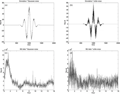
Fig. 3. The synthetic and observation smeared by the system noises. (a) Synthetic data with Gaussian noise, (b) synthetic data with white noise, (c) observation with Gaussian noise, and (d) observation with white noise.
and
B(z,t)=B0(z,t)+B0mFB ×random(z,t) (6)
whereS0andB0(z,t)are a system constant and the nature environment functions without the noises, and Fs and FB
are the amplification factors of the associated noises, re-spectively. B0m represents a reference index which is the
a tenth of maximum value of B0(z,t). Note that, in this simulation B0(z,t)is expressed by a wave packet N(z,t) of Eq. (1). The function random (in software Matlab ver-sion 5.0) returns a value between 0 and 1. To estimate the error caused by the system (nature background) noise, we
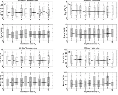
Fig. 4. Errors of the phase and group velocities computed from Fig. 3. (a) Synthetic with Gaussian noise, (b) synthetic with white noise, (c) observation with Gaussian noise, and (d) observation with white noise. The box plots of the upper and lower panels show the errors of phase and group velocities, respectively. The box plots illustrate the median value (solid line) and inter quartile range (bar) estimated by 100 calculations (dot) at various amplification factors.
noise results in much greater errors than the Gaussian. The errors of the phase and group velocities in the observation are much larger than those in the synthetic, respectively. In general, for the various amplification factors, the errors are about constants. Note that FS =1 andFB =0 is used to estimate the errors caused by intrinsic noises of MU radar.
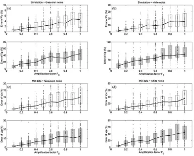
Following the similar approach, we evaluate the error owing to the nature background noise by combining Eqs. (4)–(6) and giving FS = 0 but varying FB from 1 to 10, respectively. Figure 5 displays the synthetic and observed waves mixed with two noises with a background amplifi-cation factor FB = 10. Similarly, the errors of the group velocities are larger than those of the phase velocities, and the white noise results in much greater errors than the Gaus-sian (Fig. 6). The errors of the phase and group velocities in the observation are similar to those in the synthetic, respec-tively. It is interesting to find that the larger background amplification factors yield the larger errors in the phase and group velocities.
3.
Discussion and Conclusion
It is found that the phase velocities above and below 437 km altitude are in the downward and upward directions, re-spectively, while the group velocities above and below 434– 493 km altitude are in the upward and downward directions, respectively (Fig. 1(b)). The group (phase) velocity in the away and toward direction indicates that the wave origin (or energy source) is at about 434–493 km altitude where it is
near theF2peak, upperF2region. Kelley (1989, 2009) ob-served some common features in several nights of the mid-latitude ionosphere at the Arecibo radar observatory. He reported that theF peak itself displays undulations with a period of 2 hours and the F layer rose and fell many tens of kilometers during these long-period oscillations. Kelley (2009) further cross-examines characteristics of the above features and those of atmospheric tides, and suggests grav-ity waves are probable the causal. Similarly, the MU radar observation shown in this paper reveals theF-layer electron density undulations with a period of 3–5 hours (about 224.5 minutes). Liuet al. (2007) cross-compare characteristics observed in this study with those of external factors, such as traveling ionospheric disturbances, atmospheric gravity waves, neutral winds, plasma flows, etc. Based on the ob-served phase velocity and group velocity having opposite directions Hines (1960), they also propose that the pro-nounced signature is likely to be caused by atmospheric gravity waves. Although, possible causal mechanism might not be yet fully indentified, we focus on error analyses on nature and radar system noises in deriving the phase and group velocities of vertical propagation waves by using the Fourier analysis.
C. C. HSIAOet al.: AN ERROR ANALYSIS ON NOISES IN DERIVING THE PHASE AND GROUP VELOCITIES 915
Fig. 5. The synthetic and observation smeared by the natural background noises. (a) Synthetic with Gaussian noise, (b) synthetic with white noise, (c) observation with Gaussian noise, and (d) observation with white noise.
ted power (modulated by the system) and the atmospheric medium (wave packet with natural background noise). It is clear that when the natural background is getting noisy, the associated random noise fluctuation starts growing, even competing with the wave packet amplitude. Because the natural background noise is a random function of space and time, the phase relationships between the adjacent altitudes are disturbed and become less correlated, which results in the errors of the two velocities increasing with the ampli-fication factor of natural noise accordingly. On the other hand, the system noise is simply a random function of time, and therefore the transmitted power together with its noise gives an equal weighting to each altitude, which preserves the phase relationships along the altitude. Therefore, the errors of the two velocities remain about constants and not functions of the amplification factor of the system noise.
It is found that for the system noise simulations, the er-rors of phase and group velocities in the observation are much larger than those in the synthetic data (Fig. 4), while for the natural background noise simulations the errors of phase and group velocities in the synthetic data and obser-vation are similar, respectively (Fig. 6). The received radar signal is the product of its transmitted power and the atmo-spheric medium (Eq. (4)). Since the atmoatmo-spheric medium inhabits some natural background noise, if the system noise further smears, the errors in the two velocities in the ob-servations could be much larger than those in the synthetic data (Figs. 3 and 4). By contrast, for the natural back-ground noise simulations (Fig. 5), since no system noise is involved, the phase and group velocities in the observation and the synthetic data are similar, respectively (Fig. 6).
Both the white noise and noise with Gaussian distribu-tion are examined. It is found that either in the nature back-ground or system noise simulation, the Gaussian distribu-tion constantly yields the smaller errors of the two veloci-ties than the white noise does. Note that a small value of the half width in Gaussian distribution, the random func-tion issues numbers about a constant, while the white noise function randomly gives the numbers. Therefore, the Gaus-sian distribution contributes similar amplitude of the noise fluctuations to the wave packet, which results in the smaller errors of the two velocities.
Since the system noise is not a function of altitude, the
Acknowledgments. The authors thank Professor M. Yamamoto at Research Institute for Sustainable Humanosphere, Kyoto Uni-versity, for providing the MU radar data.
References
Alcayd˙e, D.,Incoherent Scatter Theory, Practice and Science, 1995. Altadill, D., J. G. Sole, and E. M. Apostolov, Vertical structure of a gravity
wave like oscillation in the ionosphere generated by the solar eclipse of August 11, 1999,J. Geophys. Res.,106, 21,419, 2001.
Davies, K.,Ionosphere Radio, Peter Peregrinus Ltd., 1990.
Fukao, S., Y. Yamamoto, W. L. Oliver, T. Takami, M. D. Yamanaka, M. Yamamoto, T. Nakamura, and T. Tsuda, Middle and upper atmo-sphere radar observations of ionospheric horizontal gradients produced by gravity waves,J. Geophys. Res.,98, 9443, 1993.
Hines, C. O., Internal atmospheric gravity waves at ionospheric heights,
Can. J. Phys.,38, 1441–1481, 1960.
Hunsucker, R. D.,Radio Techniques for Probing the Terrestrial Iono-sphere, Springer, New York, 1991.
Kelley, M. C.,The Earth’s Ionosphere, 487 pp., Elsevier, New York, 1989. Kelley, M. C.,The Earth’s Ionosphere: Plasma Physics and Electrodynam-ics, Second Edition, ISBN 13: 978-0-12-088425-4, Academic Press, US, 2009.
Kuo, F. S., K. E. Lee, H. Y. Lue, and C. H. Liu, Measurement of vertical phase and group velocities of atmospheric gravity waves by VHF radar,
J. Atmos. Terr. Phys.,55, 1193, 1993.
Lee, C. C., J. Y. Liu, B. W. Reinisch, Y. P. Lee, and L. B. Lee, The propagation of traveling atmospheric disturbances observed during the April 6–7, 2000 ionospheric storm,Geophys. Res. Letts.,29, 12, 2002. Liu, J. Y., C. C. Hsiao, L. C. Tsai, C. H. Liu, F. S. Kuo, H. Y. Lue, and C.
M. Huang, Vertical phase and group velocities of internal gravity waves derived from ionograms during the solar eclipse of 24 October 1995,J. Atmos. Sol.-Terr. Phys.,60, 1679, 1998.
Liu, J. Y., C. C. Hsiao, C. H. Liu, M. Yamamoto, S. Fukao, H. Y. Lue, and F. S. Kuo, Vertical group and phase velocities of ionospheric waves derived from the MU radar,Radio Sci.,42, 2007.
Oliver, W. L., S. Fukao, Y. Yamamoto, T. Takami, M. D. Yamanaka, M. Yamamoto, T. Nakamura, and T. Tsuda, Middle and upper atmosphere radar observations of the dispersion relation for ionospheric gravity waves,J. Geophys. Res.,99, 6321, 1994.
Oliver, W. L., S. Fukao, M. Sato, Y. Otsuka, T. Takami, and T. Tsuda, Mid-dle and upper atmosphere radar observations of the dispersion relation for ionospheric gravity waves,J. Geophys. Res.,100, 23,763, 1995. Oliver, W. L., Y. Otsuka, M. Sato, T. Takami, and S. Fukao, A
climatol-ogy of F region gravity wave propagation over the middle and upper atmosphere radar,J. Geophys. Res.,102, 14,499, 1997.
Sato, T., A. Ito, W. L. Oliver, S. Fukao, T. Tsuda, S. Kato, and I. Kimura, Ionosphere incoherent scatter measurements with the MU radar: Tech-niques and capability,Radio Sci.,24, 85, 1989.