Time dependent dynamical systems and geophysical flows

In Partial Fulfillment of the Requirements for the Degree of

Doctor of Philosophy

California Institute of Technology Pasadena, California

2003

Preface

This thesis was submitted at theCalifornia Institute of Technologyon March 1st, 2003, as a partial fulfillment of the requirements for the degree of Doctor of Philosophy in Control and Dynamical Systems. The thesis was defended on March 12th, 2003, in Pasadena, CA, and approved by the following research committee:

Pr. Jerry Marsden,Control & Dynamical Systems, California Institute of Technology,

Pr. Richard Murray,Control & Dynamical SystemsandMechanical Engineering, California Institute of Technology,

Pr. Anthony Leonard,Graduate Aeronautical Laboratories, California Institute of Technology

Pr. George Haller,Department Mechanical Engineering, Massachusetts Institute of Technology,

Pr. Igor Mezi´c,Mechanical and Environmental Engineering, University of California - Santa Barbara.

The thesis is intended to be a complete research report. However, an effort was made to keep the chapters independent from each other to facilitate their publication. Some chapters have or will be submitted for publication in their present forms:

Lekien, F., C. Coulliette, G. Haller, J. Marsden, and J. Paduan, Optimal Pollu-tion Release in Monterey Bay Based on Nonlinear Analysis of Coastal Radar Data, Journal of Physical Oceanography, submitted.

Lekien, F., C. Coulliette, A.J. Mariano, E. Ryan, L.K. Shay, and J. Marsden, La-grangian Structures in Very High-Frequency Radar Data and Optimal Pollution Timing, Physica D, submitted.

Coulliette C., Lekien, F. Haller G., Paduan J. and Marsden J, When Should Pollution be Released? Environmental Engineering, submitted.

Lekien, F., C. Coulliette, R. Bank, and J. Marsden, Open Boundary Modal Anal-ysis (OMA): A Complete Functional Basis to Interpolate, Extrapolate and Filter Experimental Eulerian Data,Journal of Geophysical Research, in preparation.

Lekien, F., and J. Marsden, Why Warm Core Rings Are Always Anticyclonic?, Physica D, in preparation.

Lekien, F., and J. Marsden, Separatrices in High-Dimensional Phase Spaces: Appli-cation to Van Der Waals Dissociation,Journal of Chemical Physics, in preparation.

Animations related to this thesis, related papers and supporting documents and slides used during various presentations of part of this work can be found at the following address:

to Jerry Marsden and Richard Murray at the California Institute of Technologyfor their help and support, as well as to George Haller at theMassachusetts Institute of Technology, Randy Bank at the University of California, San Diegoand Igor Mezi´c at theUniversity of California, Santa Barbara.

Most of the numerical results presented in this report have been obtained using a 32 nodeBeowulf Linux alphacluster funded byCompaqand theOffice of Naval Research. Maintaining such a system at the highest performance level has been an exciting and chal-lenging task that involved many people, including Michel Tanguay, Richard Murray, Tim Colonius, Chad Coulliette, Steve Wiggins, Steve Koonin, Anthony Leonard and Manuel Fiadero.

This research was supported by two ONR grants: N00014-01-1-0208 and the AOSN project N00014-02-1-0826. I want to thank project managers Manuel Fiadero, Resa Malek-Madani and Wen Master for their enthusiasm for our projects over the past 5 years. I am grateful for the tuition and stipend generously provided by aPoincar´efellowship.

I also want to thank the staff atCaltech who maintains the facilities to a maximum level of efficiency and particularly the staff of theDepartment of Control and Dynamical Systems, including Charmaine Boyd, Betty-Sue Herrala, Siarra Walker and Harpy Hin-doyan. I am also thankful to RuthAnne Bevier, who watched our hardware network, fixed many problems and corrected numerous security problems.

In Partial Fulfillment of the Requirements for the Degree of

Doctor of Philosophy

Abstract

This thesis presents a dynamical systems approach to transport and mixing in geophysical flows. First, new algorithms are developed that allow one to study a dynamical system that is described in a variety of ways such as by means of observational data or numerical simulations of differential equations.

Next, methods available to study non-autonomous systems, such as hyperbolic trajecto-ries and Lagrangian coherent structures, are developed. These concepts are applied to examples of interests: Monterey Bay, the coast of Florida and the circulation in the North Atlantic. Combining accurate current measurements and recent developments in dynam-ical systems theory provides new and original answers to many problems, such as the minimization of the impact of released contaminants in a coastal area or the optimization of the coverage by a group of drifters.

Contents

1 Introduction 1

2 Open-Boundary Modal Analysis: A Complete Functional Basis to

Inter-polate, Extrapolate and Filter Experimental Eulerian Data 9

2.1 Introduction . . . 9

2.2 Streamfunction and Relative Vorticity . . . 10

2.2.1 State Equation Inside the Domain . . . 10

2.2.2 Boundary Conditions . . . 11

2.3 Homogeneous Solution with Inhomogeneous Boundary Conditions . . . 13

2.3.1 Homogeneous Solution Basis . . . 13

2.3.2 Boundary Function Basis . . . 14

2.4 Inhomogeneous Modes with Homogeneous Boundary Conditions . . . 15

2.5 Complete Basis . . . 15

2.6 Example: The Unit Square . . . 16

2.7 Extrapolation, Interpolation and Filtering . . . 18

2.8 Application to Monterey Bay . . . 19

2.9 Conclusion . . . 23

3 Lagrangian Coherent Structures 27 3.1 Introduction . . . 27

3.2 Lyapunov Exponent for Time-Dependent Systems . . . 28

3.3 Lagrangian Coherent Structures . . . 29

3.4 Order of Magnitude of the Exponents . . . 30

3.5 A Simple Linear Example . . . 31

3.6 Relationship between LCS and Temperature Fronts . . . 35

4 Optimal Pollution Release in Monterey Bay Based on Nonlinear Analysis

of Coastal Radar Data 39

4.1 Introduction . . . 39

4.2 High-frequency Radar Measurements . . . 41

4.3 Lagrangian Coherent Structures . . . 44

4.4 Analysis of HF Radar Data . . . 45

4.5 Prediction of Optimal Release Time Intervals . . . 47

4.6 Application to Pollution Control . . . 54

4.7 Conclusion . . . 55

5 Lagrangian Structures in Very High-Frequency Radar Data along the Coast of Florida and Automated Optimal Pollution Timing 59 5.1 Introduction . . . 59

5.2 VHF Radar Data along the Coast of Florida . . . 60

5.3 Numerical Experiments . . . 62

5.4 Lagrangian Coherent Structures . . . 66

5.5 Analysis of the Data . . . 67

5.6 Minimization of the Effect of Pollution . . . 67

5.7 An Automated Pollution Control Algorithm . . . 72

5.7.1 Prediction Algorithm . . . 72

5.7.2 Decision Algorithm . . . 78

5.8 Conclusion . . . 79

6 Why Are Warm Core Rings Always Anticyclonic? 83 6.1 Introduction . . . 83

6.2 The Model . . . 87

6.3 Lobe Dynamics and Inter-Gyre Transport . . . 89

6.4 Ring Formation . . . 92

6.5 Manifold Deformation Framework . . . 94

6.6 Warm and Cold Core Rings . . . 97

6.6.1 Anticyclonic Rings . . . 97

6.6.2 Cyclonic Rings . . . 97

6.7 Conclusion . . . 100

B Software Development: MANGEN 109

B.1 Overview . . . 110

B.2 Graphical User Interface . . . 111

B.3 Availability and Installation . . . 114

C Separatrices in High-Dimensional Phase Spaces: Application to Van der Waals Dissociation 117 C.1 The Model . . . 117

C.1.1 The Potential . . . 118

C.1.2 The Two-Dimensional Subsystem: T-ShapedHe₋I2 . . . 119

C.1.3 Phase Space Structure of the Four-Dimensional Map . . . 120

C.2 Fragmentation Dynamics for T-ShapedHe₋I2 . . . 120

C.2.1 Lobe Dynamics and Decay Rates . . . 120

C.2.2 Results . . . 122

C.3 Fragmentation Dynamics for the Full Four-Dimensional Map . . . 123

C.3.1 Theoretical Aspects of High-Dimensional Separatrices . . . 123

C.3.2 Lobe Dynamics and Decay Rates . . . 124

C.3.3 Results . . . 124

C.3.4 Comparison of Decay Rates for the Two- and Four-Dimensional Map 131 D Transport in the Restricted Three-Body Problem 135 D.1 Motivation . . . 135

D.2 Introduction to the PC3RBP . . . 136

D.3 Transport in the PCR3BP . . . 137

Chapter 1

Introduction

Over the past 10 years there has been much work in applying the approach and methods of dynamical systems theory to the study of transport in fluids from the Lagrangian point of view. Suppose one is interested in the motion of apassive tracer(e.g., dye, temperature, or any material that has a negligible effect on the flow), then,neglecting molecular diffusion, the passive tracer follows fluid particle trajectories which are solutions of

d

dtx=u(x, t), (1.1)

whereu(x, t) is the velocity field of the fluid flow,x_∈IRn, n= 2 or 3. When viewed from the point of view of dynamical systems theory, the phase space of Eq. 1.1 is actually the physical space in which the fluid flow takes place. Evidently, “structures” in the phase space of Eq. 1.1 should have some influence on the transport and mixing properties of the fluid. Aref and El Naschie [1994]; Babiano et al. [1994] provide recent reviews of this approach.

To make the connection with the large body of literature on dynamical systems theory more concrete let us consider a less general fluid mechanical setting. Suppose that the fluid is two-dimensional and incompressible. We know that the velocity field can be obtained from the derivatives of a scalar valued function,ψ(x1, x2, t), known as thestreamfunction,

as follows

d dtx1 =

∂ψ

∂x2(x1, x2, t),

d

dtx2 = − ∂ψ

∂x1(x1, x2, t), (x1, x2)∈IR 2

In the context of dynamical systems theory, Eq. 1.2 is a time-dependent Hamiltonian vector field where the streamfunction plays the role of the Hamiltonian function. If the flow is time-periodic, then the study of Eq. 1.2 is typically reduced to the study of a two-dimensional area preservingPoincar´e map. Practically speaking, the reduction to a Poincar´e map means that rather than viewing a particle trajectory as a curve in contin-uous time, one views the trajectory only at discrete intervals of time, where the interval of time is the period of the velocity field. The value of making this analogy with Hamil-tonian dynamical systems lies in the fact that a variety of techniques in this area have immediate applications to, and implications for, transport and mixing processes in fluid mechanics. For example, the persistence of invariant curves in the Poincar´e map (KAM curves) gives rise to barriers in the flow, chaos and Smale horseshoes provide mechanisms for the “randomization” of fluid particle trajectories. An analytical technique, Melnikov’s method, allows one to estimate fluxes as well as describe the parameter regimes where chaotic fluid particle motions occur. A relatively new technique, lobe dynamics, enables one to efficiently compute transport between qualitatively different flow regimes.

Dynamical systems techniques were first applied to Lagrangian transport in the con-text of two-dimensional, time-periodic flows. In recent years these techniques have been extended to include flows having arbitrary time dependence [Wiggins, 1992; Malhotra and Wiggins, 1998; Haller and Poje, 1998]. Recently, the dynamical systems approach has been extended to a number of geophysical fluid dynamics settings [Pierrehumbert, 1991a,b; Samelson, 1992; Duan and Wiggins, 1996]. These early works mainly involved kinematically defined velocity fields. Some of the first attempts to treat dynamically evolv-ing velocity fields were done by del Castillo-Negrete and Morrison [1993] and Ngan and Shepherd [1997]. They considered special kinematic cases that could be argued to be dy-namically consistent, and hence complication provided by dynamical consistency was not present [Coulliette and Wiggins, 2000].

This may not be the case when the velocity field is obtained through the solution of some fluid dynamical nonlinear partial differential equations of motion (e.g., the Navier-Stokes equations). In general, such nonlinear partial differential equations cannot be solved analytically, i.e., the right-hand side of Eq. 1.2 cannot be represented in the form of some elementary or special functions. However, they can often be solved numerically and the velocity field may be given as output of the model simulation at a discrete time sequence which may also be spatially discrete. Another way in which the right-hand side of Eq. 1.2 can be obtained is through observational methods. Modern remote sensing techniques (such as high-frequency (HF) radar arrays) have now been developed to the point where we can measure current fields at a fairly high resolution in space and time.

x

=f(

x

,t)

analytical equations

numerical simulations

observed velocities

HT, manifolds

Dynamical constraints, Optimal release time, Coverage control, ...

pips, sips, ... DLE, LCS

Figure 1.1: Different sources of input, such as analytical equations, numerical simulations and experimental data can be used to define a dynamical systems. Nevertheless, dynam-ical systems tools such as hyperbolic trajectories, direct Lyapunov exponents, invariant manifolds and lobes can be applied to any system.

is typical of coastal HF radar data1_{. Previous modal analysis methods project the data}

only onto closed-boundary modes, and then use an ad hoc procedure to add a zero-order mode to allow flow across the boundary. Open-boundary Modal Analysis (OMA) is the first method that allows flow across an open-boundary of the domain. We present the theory and a practical use of Open-boundary Modal Analysis (OMA), a complete set of eigenfunctions that can be used to interpolate, extrapolate and filter flows on an arbitrary domain with or without flow through a segment of the boundary.

Invariant manifolds, Lagrangian Coherent Structures (LCS) and Lobe dynamics pro-vide a general theoretical framework for discussing, describing and quantifying organized structures in a fluid flow and determining their influence on transport. Earlier work [Mal-hotra and Wiggins, 1998] based on small perturbation of time-independent systems, de-veloped the general mathematical framework of hyperbolic trajectories. To begin with, one can try to identifyHyperbolic Trajectories(HTs), i.e., “moving saddle points,” whose stable and unstable manifolds divide the flow into different flow regimes. However, this approach does not extend to time-chaotic system with more than one dimension. A general method due to Haller [Haller and Poje, 1998; Haller, 2000; Haller and Yuan, 2000; Haller, 2001a] and based on an extension of Lyapunov exponents will be presented in Chapter 2. The theory of the Direct Lyapunov Exponents (DLE) method is discussed in Chapter 2. DLE and other criteria-based methods can be used to visualize quickly Lagrangian Co-herent Structures (LCS) in the flow. We discuss the LCS for an analytical example and relate such structure to temperature fronts and other Lagrangian quantities of interest.

1

When studying coastal system, the boundary of the domain of interest does not necessarily correspond

to an actual shoreline. HF radar stations have a limited range and the boundary is made of a segment of

tools to determine interval of time where the impact of released contaminant is optimal. Numerical simulations in Monterey Bay are shown in Chapter 3 and we study the coast of Florida in Chapter 4. In both cases, a simple algorithm based on Lagrangian structure is able to reduce significantly the pollution and the peak of maximum concentration of pollutant generated by a numerically simulated source of pollution.

In Chapter 5, we detail and illustrate theManifold Deformation Framework (MDF). The homoclinic or heteroclinic tangle framework is available for time-periodic systems and is typically used to describe chaotic stirring and lobe dynamics in those systems. MDF is a simpler version of the heteroclinic tangle, generalized to time-chaotic systems. The concept is applied to a simple model of the North Atlantic featuring characteristic similar to those of the Gulf Stream. In particular, the model is able to reproduce the apparition of rings along the jet. As observed experimentally, some of these rings contain fluid significantly warmer or colder than the surrounding water. It has been known for many years that these so called warm-core or cold-core rings are always anticyclonic2_{. Using the MDF and}

dynamical concepts, we show that cyclonic rings can indeed not have a cold or warm core. The appendices mostly describe our software package MANGEN that was developed to produce the results shown in this thesis. Appendix B describes the latest developments of MANGEN and its graphical user interface. Major efforts were made to write a portable library of tools that can be used in many different problems. As an example, Appendix C uses MANGEN to study transport in a higher-dimensional systems. In this example inspired by Gillilan and Ezra [1991], anHeatom interact with a Van der Waals potential created by a I2 oscillator. Wang-Sang Koon, Shane Ross and Jerry Marsden recently

pointed out that algorithms similar to those of MANGEN could be applied to the study of 3-body problems [Koon et al., 2000, 2001a,b]. Appendix D details a restricted 3-body problem and gives an overview of manifolds and transport in such systems.

2

Cyclonic rings turn in the same direction as their containing gyre. Anticyclonic rings turn in the

Once you let the Ocean take you, there is no limit to the number of amazing and intriguing places where you may drift.

Chapter 2

Open-Boundary Modal Analysis: A Complete

Functional Basis to Interpolate, Extrapolate

and Filter Experimental Eulerian Data

In collaboration with C. Coulliette, R. Bank and J. Marsden.

2.1

Introduction

In the last few years, technological advances in techniques such as high-frequency radar data provided us with fairly accurate measurements of the velocity vectors in certain coastal areas (see Coulliette and Wiggins [2001]; Lekien et al. [2003], for example). How-ever, this data cannot be used directly as a dynamical systems, unlike a smooth ordinary differential equation (ODE) that can be integrated. For instance, there are missing gaps due to the radar range and wind conditions. As a result, oceanographers are in need of a way to extrapolate, interpolate and filter such data. The resulting smooth velocity field is often called nowcastin reference to the much more common forecasting operation. Now-casting does not involve the extrapolation of the velocities in the future. It uses available data to determine the velocity everywhere in space at the same time data was collected.

side and an artificial boundary in the sea resulting from the limited range of action of the radar-antenna system. In such case, one needs to take into account the fact that portions of the boundary are permeable to water.

Many patches [Lipphardt et al., 2000] are available today to standard modal analysis techniques but they require an exact knowledge of the flux on the open-boundary. We present in this chapter a complete functional basis that can be used to project the flow on modes allowing flux through some segments of the boundary.

The method presented in this chapter is very similar to the method described in Lip-phardt et al. [2000]. The fundamental difference is the addition of an infinite (possibly truncated) sequence of boundary modes allowing adequate degrees of freedom to project the experimental data on open-boundaries. Unlike other methods, the approach we high-light renders eigenfunctions on an unstructured (triangular) mesh with a general boundary.

2.2

Streamfunction and Relative Vorticity

2.2.1

State Equation Inside the Domain

The velocity nowcast will be referred to by a function ¯uof a compact set Ω_∈R2_{. If Ω is}

simply connected and its boundary is piecewise smooth, the Hodge decomposition [Eise-man and Stone, 1973] states that ¯ucan be written as the sum

¯

u= ¯uψ+ ¯uφ, (2.1)

where

¯

uψ =∇ ×ψk,¯ (2.2)

is divergence-free and

¯

uφ=∇φ, (2.3)

is irrotational. Combining Eqs. 2.2 and 2.3 with Eq. 2.1 gives

¯

u=_{∇ ×} ψ¯k

+_∇φ, (2.4)

where ¯kis the unit vector orthogonal to the domain, pointing upwards. Applying∇·and

∇×to Eq. 2.4 gives

∆ψ=₋¯k_·(_{∇ ×}u¯). (2.6)

2.2.2

Boundary Conditions

We will let ∂Ω denote the boundary of the compact domain Ω. The unit vector normal to the boundary∂Ω and pointing outward the domain is denoted by ¯n(Fig. 2.1 (a)). The unit tangent vector is ¯t = ¯n_×k¯. We assume that the boundary ∂Ω is continuous and piecewiseC1_{(i.e., for all but a finite number of pointsxon the boundary, there exists an}

open set Uxcontainingxsuch thatUx∩∂Ω is then graph of aC1 function). Multiplying

Eq. 2.4 by either ¯tor ¯ngives

¯

u_·¯t = ¯t_{· ∇ ×}ψ¯k + ¯t._∇φ

= ¯t_{· ∇}φ+ ¯n_{· ∇}ψ, (2.7)

and

¯

u·¯n = n¯· ∇ ×ψ¯k

+ ¯n.∇φ

= n¯· ∇φ−_t¯_{· ∇ψ,} (2.8)

which can be used to establish the boundary conditions on the scalar functionsφandψ. We will now assume that the boundary∂Ω is made of the union of two different boundary pieces

  

∂Ω =∂Ω0∪∂Ω1

∂Ω0∩∂Ω1=∅,

(2.9)

where∂Ω0is a portion of real boundary (the shoreline) and∂Ω1 is an artificial boundary

through which a flux might exist (see Fig. 2.1 (b)). ∂Ω1 is included in our derivation

because the basin of fluid may be too large to include the whole area in the computation. The user may have some measurements in a coastal area and cannot define Ω as the whole ocean. Instead he will join a segment of the real coastline∂Ω0to an artificial boundary∂Ω1

(called the open-boundary) in the ocean to close the domain of interest. If∂Ω =∂Ω0 our

W

W

t

n

k

W

W

0

W

1

coastline

(a) (b)

Figure 2.1: (a) Domain Ω and its boundary ∂Ω. ¯k is the unit vector orthogonal to the ocean surface, pointing up to the reader. ¯n is the unit vector normal to the boundary

∂Ω and the tangent vector is defined as ¯t= ¯n×k¯. (b) The portion∂Ω0 is made of solid

ground and has no normal flow while∂Ω1 is subject to an arbitrary flux.

Eq. 2.7 and 2.8 are not sufficient to establish boundary conditions for the two functions

φandψ. However, the decomposition given by Eq. 2.1 is not unique. Given a particular solution, one can add a divergence-free function toφand a zero vorticity term toψ. This degree of freedom allows us to make the following choice onφandψ: The incompressible ¯

uψ part does not produce any flux through∂Ω0, i.e.,n¯·u¯ψ=−¯t· ∇ψ= 0.

This is a very natural choice in the sense that if the boundary was completely of type

∂Ω0, we would requireψ= 0 on the boundary (see [Eremeev et al., 1995b,a] or [Lipphardt

et al., 2000] for example) which implies ¯t· ∇ψ= 0.

As a result, the second term of Eq. 2.8 disappears on∂Ω0 and gives

¯

n_{· ∇}φ = u¯_·n¯ on∂Ω0

= 0 on∂Ω0,

(2.10)

where we used the fact that ¯u.n¯= 0 on∂Ω0. We assume that∂Ω0is connected in∂Ω, i.e.,

there is only one connected segment of shoreline (see Fig. 2.1 (b), for example). Since we have ¯t._∇ψ= 0 on the segment∂Ω0 and ψcan be added any arbitrary constant function

and _        

∆ψ=₋¯k.(_{∇ ×}u¯) in Ω, ψ= 0 on∂Ω0,

ψ=gψ(s) on∂Ω1,

(2.12)

where gφ(s) and gψ(s) are two unknown L2(∂Ω1) functions of the arclength s on the

boundary that depend on the velocity field ¯u. We can also write the problem in the following way

  

∆φ=_{∇ ·}u¯ in Ω,

¯

n· ∇φ=gφ(s) on∂Ω,

(2.13)

and _

 

∆ψ=−k¯(∇ ×ψ) in Ω, ψ=gψ(s) on∂Ω,

(2.14)

where we implicitly mean thatgφ andgψ vanish on∂Ω0.

2.3

Homogeneous Solution with Inhomogeneous

Bound-ary Conditions

The boundary modes or homogeneous modes are obtained by solving the homogeneous problem with inhomogeneous boundary conditions

  

∆φb −R

∂Ωgφ(s)ds= 0 in Ω,

¯

n_{· ∇}φb_=g

φ(s) on∂Ω,

(2.15)

2.3.1

Homogeneous Solution Basis

We assume that the set _F of scalar functions on the boundary with support included in

Figure 2.2: The parameter s is the arclength on the boundary and is defined in such a way that the open-boundary runs froms = 0 to s=l. The remainder of the boundary (s > l) is the shoreline.

of the basis functiongi. Let us defineφbi to be the solution of the problem

  

∆φb i−

R

∂Ωgi(s)ds= 0 in Ω,

¯

n_{· ∇}φb

i =gi(s) on∂Ω.

(2.16)

Providing that we add a condition such as

Z Z

Ω

φbids= 0, (2.17)

the solutions ψb

i of Eq. 2.16 are unique. Indeed, this is seen by a standard argument.

Suppose thatφb i andφ

0_b

i are two solutions for Eq. 2.16 with the same gi on the boundary.

Their differenceδ=φ0b

i −φbi must satisfy

  

∆δ= 0 in Ω,

¯

n_·δ= 0 on∂Ω. (2.18)

Eq. 2.17 and 2.18 givesδ= 0. Therefore,φb

i is unique.

2.3.2

Boundary Function Basis

A natural choice is a discrete Fourier basis of the function defined on the open-boundary

{gi(s)}=

1, . . . ,sin iπ l s ,cos iπ l s , . . . , (2.19)

2.4

Inhomogeneous Modes with Homogeneous

Bound-ary Conditions

The inhomogeneous modes satisfy the following equations

  

∆φi=λφiφi in Ω,

¯

n._∇φi= 0 on∂Ω,

(2.20)

  

∆ψi=λψiψi in Ω,

ψi= 0 on∂Ω,

(2.21)

whereλφ_i andλψ_i are the (unknown) eigenvalues andφi andψi are the eigenfunctions.

According to Appendix A.4, the modes _{φi} and {ψi} form a basis of respectively

W1_{(Ω) and W}1

0(Ω). As a result, the associated vector fields {∇φi} and {∇ ×ψi} span,

respectively, the spaces

¯

u_∈L2(Ω)_×L2(Ω)

∇ ×u¯= 0 and ¯n.∇u¯|∂Ω = 0 , (2.22)

and

¯

u_∈L2_(Ω)

×L2_(Ω)

∇.u¯= 0 and∇n.¯u¯|∂Ω = 0 (2.23)

Using the Hodge decomposition and the associated remark in Section 1, we conclude that the inhomogeneous modes{∇φi,∇ ×ψi}span the set

¯

u_∈L2(Ω)_×L2(Ω)

∇n.¯u¯|∂Ω = 0 (2.24)

2.5

Complete Basis

The nowcast velocity is given by a function ¯uon Ω such that each component belongs to

L2_{(Ω) and ¯usatisfies the boundary condition ¯n.u¯ = 0 on∂Ω}

0. We assume that we have

by

g(s) = ¯n.u¯|∂Ω (2.25)

Since_{gi} is a basis ofL2[0, l], we can expandg as

g=

∞

X

i=1

αb

igi, (2.26)

We define

¯

uH = ¯u− ∞

X

i=1

αbi∇φbi (2.27)

and we remark that ¯uH

∈L2_{(Ω) satisfies the homogeneous boundary conditions. In other}

words, ¯uH _{does not generate normal flow on either∂Ω}

0and ∂Ω1. As a result, ¯uH can be

written as a unique sequence of homogeneous modes

¯

uH =

∞

X

i=1

αψi∇ ×ψHi + ∞

X

i=1

αφi∇φHi , (2.28)

and the velocity nowcast can be written as a unique sequence

¯

u=

∞

X

i=1

αψ_{i∇ ×}ψi+ ∞

X

i=1

αφ_i∇φi+ ∞

X

i=1

αb

i∇φbi. (2.29)

When the fluid is incompressible, the nowcast can be obtained with the incompressible modes only, because the projection on the other modes must vanish. Using only incom-pressible modes guarantees that the resulting nowcast will be incomincom-pressible. Assuming that the (finite or infinite) sequence of boundary modes that are incompressible isnφb

βi

o , the nowcast ¯uH can be written using the truncated sequence

¯

u=

∞

X

i=1

αψ_{i∇ ×}ψi+ ∞

X

i=1

αbβi∇φ b

βi. (2.30)

2.6

Example: The Unit Square

We consider the following domain

Figure 2.3: Sample domain for OMA modes. The domain Ω is the unit square. The eastern side of the square (∂Ω1) is open and allow arbitrary flux. The three other sides of

the square constitute the shoreline∂Ω0.

where

∂Ω0 = {0≤x <1 andy= 0}

∪ {0≤x <1 and y= 1} ∪ {0≤y≤1 and x= 0},

(2.32)

is the solid boundary (land) and

∂Ω1={0≤y≤1 and x= 1}, (2.33)

allows transport (see Fig. 2.3). The inhomogeneous modes are given by:

ψk,l = sin(kπx) sin(lπy),

φk,l = cos(kπx) cos(lπy),

(2.34)

and the associated velocity modes

¯

uψ_k,l=∇ ×ψk,l = π

 

ksin(kπx) cos(lπy)

−lcos(kπx) sin(lπy)  ,

¯

uφk,l=∇φk,l = −π

 

ksin(kπx) cos(lπy)

lcos(kπx) sin(lπy)  ,

(2.35)

modes. We illustrate the process by computing the modes corresponding to

gk(s) =gk(y) =πcos(kπy). (2.36)

One can verify that the unique solution to Eq. 2.16 is

φbk =

ekπx_+e−kπx

ekπ_−e−kπ cos(kπy), (2.37)

and the corresponding boundary modes are

¯

ub

k =∇.φbk =

1

k

 

ekπx_−e−kπx

ekπ_−e−kπ cos(kπy) −ekπx_+e−kπx

ekπ_−e−kπ sin(kπy)



 (2.38)

Forgk(y) = sin(kπy), we could not find an analytical solution, only a numerical one.

A detailed algorithm to compute OMA modes can be found in Section 2.8.

2.7

Extrapolation, Interpolation and Filtering

Eq. 2.29 can be rewritten in the more compact form

¯

u=

∞

X

n=1

αn¯un, (2.39)

where ¯un represent any of the linearly independent modes (boundary, incompressible or

irrotational). Since the sequence of mode is infinite, the optimal coefficients αn cannot

be determined with a finite number of measurements. However, the smaller details are obtained for high eigenvalues and using a finite sequence as an approximation to Eq. 2.39 allows to filter the data and keep significant details only. The nowcast at a particular time is given by

¯

u0=

N

X

n=1

αnu¯n, (2.40)

whereN is the total number of modes (rotational, incompressible and boundary) and ¯un

represent any of these linearly independent modes.

If we were using all the modes, the error on ¯u will be zero but that would require an infinite number of measurements to determine the infinite number of coefficients αn.

q

to minimize is

= v u u t X q X n

αnu¯n(¯xq)−u¯mesq

2 , (2.41)

where the norm can be_kk2 to get a least square minimization problem or any other norm depending on the user choice. A set of projection coefficientsαiminimizes the error, when

∂

∂αj = 0,∀j, (2.42)

or X n αn X q

(¯un(¯xq).u¯j(¯xq)) =n

X

q

¯

umesq .u¯j( ¯xq),∀j. (2.43)

Eq. 2.43 is a linear system of k equations withN unknowns αi. Usually, the number of

modes N is much smaller than the number of measurementsk and the linear system is over-determined. Many algorithms are available to find the solution of over-determined systems that minimizes the residue and most of them have a portable implementation. Here, we use theGNU Scientific Library1_.

2.8

Application to Monterey Bay

This application uses high-frequency (HF) radar technology [Paduan and Rosenfeld, 1996; Paduan and Cook, 1997; Prandle and Ryder, 1985; Goldstein and Zebker, 1987; Georges et al., 1996], which is now able to resolve time-dependent Eulerian flow features in surface currents along coastlines. Such a HF radar installation has been operating in Monterey Bay since 1994 [Paduan and Rosenfeld, 1996; Paduan and Cook, 1997]. In our study, we use data from this installation, acquired by the three HF radar antennas near Monterey Bay, CA. The observational data was collected in August 2000, binned every hour on a uniform grid with 1 km by 1 km intervals. An example of an HF radar footprint of the Bay at 05:00 GMT, August 12, 2000 is shown in Fig. 2.4. Also shown on Fig. 2.4 are the level sets of the percentage of available data in the bay for the month of August 2000. There

1

Figure 2.4: The black vectors show a footprint of the HF radar data in Monterey Bay on August 15 12:00 GMT. Also shown on this picture are the level sets of the percentage of available data during the month of August 2000. Regions in red have data almost all the time. Data is almost unavailable most of the time in the blue regions.

are many gaps in the data. Moreover, the missing data points are always located in the same region. The reason for this distribution is the range of the radar. The performance decreases with the distance. Also, some regions do not have ripples with enough amplitude to scatter the waves and the radar cannot determine the velocity. Our objective is to build an extrapolation method that filters and extrapolate such incomplete data sets.

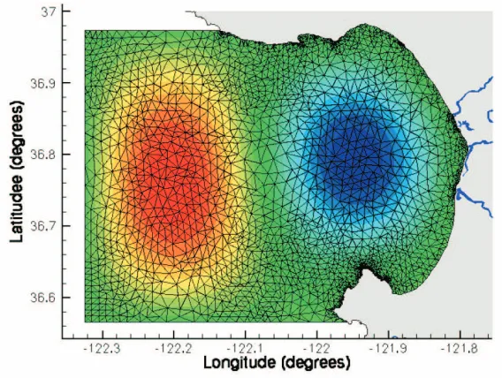
A high-precision version of the shoreline for our domain was extracted on a topological map and is visible on Fig. 2.4. We used a numerical software package calledP LT M G2 _to

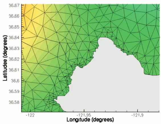
solve the mode equations (Eq. 2.20, 2.21 and 2.16). Fig. 2.5 shows a particular instance of the adaptive mesh used to compute one of the modes. The use of an unstructured mesh is necessary for applications such as the integration of particle or the computation of s Lagrangian structure near a complicated shoreline. Inadequate representation of the shoreline or a lack of precision in the velocity field near the coast often results in particles erroneously crossing the shoreline. Fig. 2.6 shows the unstructured mesh in a magnified region centered on Point Pinos, the southernmost part of the bay featured on Fig. 2.5, where separation of the flow between the bay and the ocean occurs. Fig. 2.7 shows the computed streamlines and velocities in the Point Pinos area. Such precise streamlines

2

Figure 2.5: Adaptive mesh used for the computation of the 2nd incompressible modeψ2.

cannot be obtained with a structured mesh.

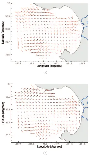
Fig. 2.8 shows two nowcasts realized with OMA. The upper nowcast uses only four incompressible modes and four irrotational modes. It cannot produce any flow normal to the boundary. It is similar to the nowcasts obtained after the first two steps of the algorithm described in [Lipphardt et al., 2000]. The lower nowcast uses eight boundary modes and is able to generate normal flow on the open-boundary (interaction with the Pacific ocean). As a result, the error between the HF radar data (red arrows on Fig. 2.9) and the nowcast, that does not use boundary modes (black arrows on Fig. 2.9), can be extremely large near the open-boundary. Fig. 2.9 also reveals that including 8 boundary modes in the nowcast decreases the error significantly near the open-boundary.

Figure 2.6: Unstructured mesh near Point Pinos, the southernmost point of the bay where the flow separates between the bay and the Pacific ocean.

(a) (b)

(a) (b)

Figure 2.8: Comparison between NMA and OMA nowcast on July 7, 2000 at 09:00 GMT. Both nowcasts use 4 incompressible modes and 4 irrotational modes. (a) does not use any boundary and cannot produce any flow through the open-boundary. (b) uses 8 boundary modes.

2.9

Conclusion

We presented a practical method to interpolate, extrapolate and filter experimental Eule-rian data. This is the first modal analysis that includes a sequence of boundary modes. As a consequence, the modeler does not need to speculate on the open-boundary flux. Previous approaches [Lipphardt et al., 2000] require the use of a larger model or some assumptions to determine the flux through the open-boundary. In contrast, OMA adapts the flow near the boundary with the available data through Eq. 2.43. If the normal flow is known near the boundary, OMA uses this information and provides nowcasts similar to the adapted three-step algorithm in Lipphardt et al. [2000]. If, at some time, data is available only in the middle of the domain, far away from the boundary, OMA naturally projects the data on the boundary modes and finds the boundary flow that best fits the data.

(a)

(b)

(a) (b)

Figure 2.10: Comparison between NMA and OMA nowcast on July 17, 1999 12:00 GMT. (a) uses 4 incompressible modes and 4 irrotational modes. (b) uses 4 additional boundary modes. Only the OMA nowcast (a) is able to reproduce the separation point on the shoreline (near Point Pinos) that was visible in the HF radar data. Certain important dynamical features can be wiped by removing the boundary modes.

at a constant rate (∆T), OMA provides the nowcast as a sequence of coefficients

                          

α1(t0), α1(t0+ ∆T), ... , α1(t0+i∆T), ...

α2(t0), α2(t0+ ∆T), ... , α2(t0+i∆T), ...

...

αk(t0), αk(t0+ ∆T), ... , αk(t0+i∆T), ...

...

αN(t0), αN(t0+ ∆T), ... , αN(t0+i∆T), ...

(2.44)

Knowingαp_k(t0+i∆T) fori= 1→N, one can predict the evolution of the coefficient for

Chapter 3

Lagrangian Coherent Structures

In collaboration with George Haller.

3.1

Introduction

A “moving” invariant manifold or material line can be defined as a time-dependent curve

f(x, y, t) = 0 ∀t, (3.1)

such that

∂f ∂xx˙+

∂f ∂yy˙=−

∂f

∂t. (3.2)

It is not easy to define the equivalent of hyperbolic fixed points and stable or unsta-ble invariant manifolds for time-dependent systems. The definition of “moving” invariant manifold can be used to define attracting or repelling lines in the flow, but most mate-rial lines are only hyperbolic for finite time. As a result the intersection, of those lines are hyperbolic trajectories only during short interval of times. More dramatically, some attracting lines become gradually less important and new attracting lines take over the general behavior of the flow. In some sense, it is hopeless to try to determine “the most influential” hyperbolic trajectories, because the influence of each trajectory changes over time.

Lagrangian structures in a flow. We then illustrate the method with a linear examples and discuss the sensitivity of Lyapunov exponents to anomalies in the flow.

3.2

Lyapunov Exponent for Time-Dependent Systems

A trajectory starting at time t0 at the position x0 is located at the position x(t;t0,x0)

after a time (t₋t0). The Lyapunov exponents of this trajectory are related to the norm

of a perturbation of the trajectory. Let us assume that we perturb the initial condition to x0+δx. For infinitesimal perturbation δx(0), the position at time t of the perturbed

trajectory will be given by

x(t;t0,x0) +δx(t), (3.3)

where

δx(t) =

∂x(t;t0,x0)

∂x0

δx(0), (3.4)

and the norm of the perturbation becomes

kδx(t)k2=δTx(0)

_∂x(t;t

0,x0)

∂x0

T _∂x(t;t

0,x0)

∂x0

δx(0). (3.5)

Let us define the Cauchy-Green strain tensor by

S(t;t0,x0) =

_∂x(t;t

0,x0)

∂x0

T _∂x(t;t

0,x0)

∂x0

, (3.6)

which allows us to rewrite Eq. 3.5 as

kδx(t)k2=δTx(0)Sδx(0). (3.7)

The Lyapunov exponents are typically defined as the limit fort_→+_∞of (1/t₋t0) times

the logarithm of the eigenvalues of

∂kδx(t)k

∂_kδx(0)k

= 1

2

√

S, (3.8)

Σ(t;t0,x0) =

1 2

1

t−t0

lnS(t;t0,x0), (3.10)

and the Lyapunov exponentsσ1 andσ2 are given the eigenvalues of

lim

t→∞Σ(t;t0,x0). (3.11)

3.3

Lagrangian Coherent Structures

We take the largest singular valueσt(x0, t0) of the derivative of the flow map with respect

tox0. More specifically, we calculate the scalar fieldσt(x0, t0) as the largest eigenvalue of

the Cauchy-Green strain tensor. As argued in Haller [2001a], repelling material lines are local maximizing curves ofσt(x0, t0), which will allow us to capture these material lines at

timet0as ridges of the scalar fieldσt(x0, t0). The same procedure performed in backward

time (i.e., fort < t0) would render attracting material lines as ridges ofσt(x0, t0).

This algorithm takes into account Lagrangian hyperbolicity and is not based on in-stantaneous approximation of the Cauchy-Green tensor. The convergence time (t₋t0)

in Eq. 3.10 is an important parameter. It makes the Direct Lyapunov Exponent algo-rithm different from Lyapunov exponents (obtained fort_→+_∞). We know that a small convergence time will not produce satisfying results as it will not be Lagrangian enough (an Eulerian approximation can be computed fort =t0. On the other hand, looking at

infinite-time may not be the more efficient way to study non-autonomous systems. These can indeed switch between different dynamical modes or oscillate between different be-haviors. An optimal convergence timet₋t0 needs to be determined for each application

and the type of information seek (short or long term analysis and prediction). The next chapter includes a discussion about the minimum timet₋t0that can be used for a specific

application.

3.4

Order of Magnitude of the Exponents

We would like to show that factor (t−t0)−1 in Eq. 3.10 is important for numerical

sta-bility and also allow us to compute an approximation ofσ. The analogy with Lyapunov exponents insures that the limit

lim

t→+∞σ(t;t0,x0), (3.12)

converges and is equal to the Lyapunov exponent of the trajectory starting atx0 at time

t0. Omitting (t−t0)−1 creates an overflow problem, since

Eig_{lnσ(t;t0,x0)} ∼(t−t0), (3.13)

Under an infinitesimally small timeδt, a trajectory starting atx0 at timet0moves to

x(t) =u_|x0δt. (3.15)

A perturbed trajectory starting att0in x1=x0+δx moves to

x0+δx+u|x0δt+J|x0δxδt, (3.16)

and the instantaneous perturbation is given by

δx(δt) =J|x0δx(0)δt. (3.17)

Its growth is given by

kδx(δt)_k=δx(0)JJT

_x0δx(0)δt, (3.18)

and an approximation of the Lyapunov exponents are given by the eigenvalues of

S(t;t,x0) =JT(x0, t)J(x0, t). (3.19)

3.5

A Simple Linear Example

We will apply the previous results to the “rotating saddle” defined by

˙

x=

 

cos 2ωt sin 2ωt

sin 2ωt ₋cos 2ωt



x. (3.20)

This system is linear and admits a stagnation point x = 0. The eigenvalues are con-stant and equal to +1 and₋1 and the system admits 2 eigenvectors associated with each eigenvalue

e+1=

 

cosωt

sinωt



x

y

ω

=0.5

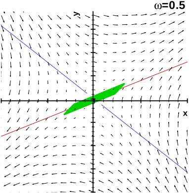
Figure 3.1: The rotating saddle forω = 1₂. There exists a stable (blue) and an unstable (red) invariant manifold attached to the fixed point. A parcel (green) integrated will slowly spread to the unstable manifold.

and

e−1=

 

−sinωt

cosωt



. (3.22)

The eigenvectors are rotating with a constant angular speed ω. For ω = 0 and ω small enough, we expect to find two invariant manifolds, one of each stability type. This situation is depicted in Fig. 3.1 forω= 1/2. We remark that the invariant manifolds arenot aligned with the instantaneous eigenvectors. The unstable manifold is shifted by an angleφbehind thee+1 and the stable manifold is in advance with respect toe−1with the same angleφ.

The angleφcan be found as the solution of

sin 2φ=ω. (3.23)

Not surprisingly, Eq. 3.23 does not admit any solution when the rotation speedωbecomes too large. In that case, the rotating saddle behaves more like a center. Fig. 3.2 illustrates this phenomenon forω= 3/2.

Fig. 3.3 shows that when the rotation speed of the eigenvectors is not too large, the max-imum ridge of the fieldσcaptures the stable manifold of the system. Plottingσ(₋t;t0,x0)

x

Figure 3.2: The rotating saddle for ω = 3₂. Even though the rotating saddle has a stable eigenvector with constant eigenvalue₋1 and an unstable eigenvector with constant eigenvalue +1, the system does not have stable or unstable invariant manifold attached to the saddle because its eigenvectors are turning too fast. The trajectory at the origin isnot hyperbolic and a parcel starting near the origin does not reveal any hyperbolic behavior.

x

y

ω

=0.5

x

y

ω

=1.5

Figure 3.4: Direct Lyapunov Exponent Algorithm for the Rotating Saddle with ω = 3

2.

Theoretically, the Lyapunov exponent is constant in space. The weak contrast and the angles are artifacts of neglecting trajectories outside the box.

Fig. 3.4 reports the same computation for ω = 3/2. We can see that the DLE plot reveals no Lagrangian structure, as there are no stable or unstable manifolds.

gorithm. Past successful efforts have been using the Thermal Front Parameter (TFP) defined as

τ=_−∇(_|∇T_|) ∇T

|∇T_|. (3.24)

The TFP magnitude is large when there is a rapid change in the thermal gradient with a large component parallel to the direction of the (unitized) thermal gradient. If we restrict the system to a one-dimensional problem, a line parallel to the gradient of the temperature, this means that the second derivative ofT is zero, i.e., the temperature “stops to increase dramatically.” The minus sign is a convention and place the frontal boundary on the warm side of the concentrated level sets (ridge line in the field of TFP). Similarly, using −τ would detect cold fronts.

Longitude (degrees) L a ti tu d e (d e g re e s )

-122.2 -122.1 -122 -121.9 -121.8

36.6 36.7 36.8 36.9 37

Figure 3.5: DLE field for the ICON model of Monterey Bay. A black line indicates the position of a DLE front.

Longitude (degrees) L a ti tu d e (d e g re e s )

-122.2 -122.1 -122 -121.9 -121.8

36.6 36.7 36.8 36.9 37

Longitude (degrees)

L

a

ti

tu

d

e

(d

e

-80.125 -80.1 -80.075 -80.05 -80.025

26.02 26.03 26.04 26.05 26.06

Figure 3.7: Average velocity in thexdirection orx-patchiness plot for the RSMAS domain depicted in Chapter 5.

3.7

Other Methods

Extracting material lines in time-dependent flows is a complex problem and has been studied for many years. In this thesis we use mainly the method of the Direct Lyapunov Exponents. However, many other criteria have been used over the past. Early works [Mal-hotra et al., 1998; Poje et al., 1999] used the averagexandy components of the velocity. We computed these fields (see Fig. 3.7 and 3.8), also called patchiness plots, for the small domain near the coast of Florida depicted in Chapter 5. The LCS extracted from the DLE plot (Fig. 3.9) corresponds exactly to the dividing line in the patchiness plots.

Longitude (degrees) L a ti tu d e (d e g re e )

-80.125 -80.1 -80.075 -80.05 -80.025

26.02 26.03 26.04 26.05 26.06 26.07 26.08 26.09 26.1

Figure 3.8: Average velocity in theydirection ory-patchiness plot for the RSMAS domain depicted in Chapter 5.

Longitude (degrees) L a ti tu d e (d e g re e )

-80.125 -80.1 -80.075 -80.05 -80.025

26.02 26.03 26.04 26.05 26.06 26.07 26.08 26.09 26.1

Chapter 4

Optimal Pollution Release in Monterey Bay

Based on Nonlinear Analysis of Coastal

Radar Data

In collaboration with Chad Coulliette, George Haller, Jeffrey Paduan and

Jerry Marsden.

4.1

Introduction

The release of pollution in coastal areas [Prahl et al., 1984; Rice et al., 1993; Verschueren, 1983] can lead to dramatic consequences for local ecosystems if the pollutants recirculate close to the coast rather than being transported out to the open ocean, where they are dispersed and then absorbed. This article shows how a combination of accurate current measurements and recent developments in nonlinear dynamical systems theory uncovers previously unknown flow structures that govern mesoscale ocean mixing. Knowledge of these Lagrangian (i.e., material) structures1 _{can lead to predictions on a number of}

phe-nomena, ranging from the motion of plankton populations to the evolution of oil spills. The present article shows how Lagrangian flow structures can be exploited to reduce the dam-aging effects on coastal pollution. The focus of our study is the Elkhorn Slough, located near Moss Landing harbor of Monterey Bay. The Elkhorn Slough is a regular source of or-ganic contaminants such as dichlorodiphenyl-trichloroethane (DDTs) and polychlorinated biphenyl (PCBs) from agricultural run-off, phthalic acid esters (PAEs) from plasticizer manufacturing, insecticidal sprays, wetting agents and repellents, and polycyclic aromatic

1

hydrocarbons (PAHs) from the combustion of natural fossil fuels [Prahl et al., 1984; Rice et al., 1993; Verschueren, 1983].

Note that unlike other articles on pollution in this region, we are not implying that there is a pollution problem in Monterey Bay, but rather that predicting the optimal time window can significantly reduce the damage done in the coastal region by any amount of pollution, whether it is a small trickle from a stream or a huge oil spill from a tanker. For Monterey Bay, we will specifically show that surface current observations from coastal radar antennas located near Monterey Bay can be used to reduce the time which the aforementioned contaminants spend in the bay, and thus reduce the damage caused to the environment.

We examine high-frequency (HF) radar measurements [Paduan and Rosenfeld, 1996; Paduan and Cook, 1997; Prandle and Ryder, 1985; Goldstein and Zebker, 1987; Georges et al., 1996] of near-surface currents in Monterey Bay, and identify an LCS that governs the chaotic mixing of any Lagrangian particles, in this case we are specifically interested in Lagrangian contaminants over finite intervals of data. Specifically, we find a highly convoluted LCS— composed of a line of fluid particles— that repels nearby fluid parcels and hence acts as a barrier between two different types of motion: recirculation and escape from the bay. Release of pollution on one side of this moving fluid structure will result in sustained recirculation of the contaminant in the bay. If, however, pollution is released on the other side of the repelling material line, then the contamination will quickly clear from coastal regions and head towards the open ocean. Clearly, the latter scenario is highly desirable, while the former is to be avoided. We propose an algorithm that uses real-time HF radar data to predict release times leading to the desired pollution behavior.

A similar approach should work for optimizing the release of pollution into the atmo-sphere, rivers, lakes, or other waterways in any situation where sufficiently accurate wind or current velocity data is available, and the release of pollution can be contained until an appropriate release time. HF radar has also been demonstrated to work equally well in fresh water areas, but typically higher frequencies are necessary for the smaller regions, thus it is called Very High-Frequency (VHF) radar.

2001]. The presence of coherent features in measured geophysical flow data prevents the application of homogeneous and isotropic turbulence theory [Coulliette and Wiggins, 2000; Fischer et al., 1979] while the temporal irregularity and spatial complexity of such data renders the classic techniques of chaotic advection inapplicable [Watson et al., 1999; Zimmerman, 1986; Ridderinkhof et al., 1990; Beerens et al., 1998].

4.2

High-frequency Radar Measurements

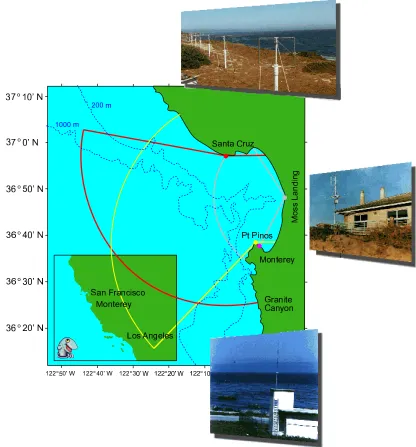
Our analysis makes use of high-frequency (HF) radar technology [Paduan and Rosenfeld, 1996; Paduan and Cook, 1997; Prandle and Ryder, 1985; Goldstein and Zebker, 1987; Georges et al., 1996], which is now able to resolve time-dependent Eulerian flow features in surface currents along coastlines. Such an HF radar installation has been operating in Monterey Bay since 1994 [Paduan and Rosenfeld, 1996; Paduan and Cook, 1997]. In our study, we use data from this installation, acquired by the three HF radar antennas shown in Fig. 4.1. binned every hour on a horizontal uniform grid with 1 km by 1 km intervals. An example of an HF radar footprint of the Bay at 05:00 GMT, August 12, 2000 is shown in Fig. 4.2.

We describe fluid particle motion in Monterey Bay as a dynamical system obeying

˙

x=v(x, t). (4.1)

To determine the velocity, the left-hand side of Eq. 4.1, we examine high-frequency (HF) radar measurements of near-surface currents in Monterey Bay. Ignoring measurement errors, the HF data is a footprint of the actual velocity in the bay as described by Eq. 4.1. The temporal complexity of the currents becomes evident from tracking different evolutions of a fluid parcel—a model for a blob of contaminant— released at the same precise location, but at slightly different times. We show the results of two such numerical experiments in Fig. 4.3.

Figure 4.2: Instantaneous near-surface velocities (white arrows) at 08:00 GMT, August 8, 2000, obtained from the three HF antennas in Monterey Bay. Blue circles indicate all locations where continuous measurements were binned.

Runge-Kutta algorithm combined with third-order polynomial interpolation in time and bi-cubic interpolation in space. We used these particle trajectories to approximate the flow map, which associates current positions to flow positions. We modelled the coastline as a free-slip boundary, and disregarded particles that crossed the linear fluid boundaries of the domain on the northern, southern and western edges. All these numerical algorithms have been compiled into a software package, MANGEN2_{, described in Appendix B.}

Note that the black contaminant parcel remains in the bay, whereas the white parcel exits the bay and moves towards the open ocean. The latter scenario is highly desirable, because it minimizes the impact of the contaminant on coastal waters, by causing it to be safely dispersed in the open ocean. This observation inspires us to understand and predict different evolution patterns of the same fluid parcel, depending on its initial location and time of release. Such patterns are known to be delineated by attracting material lines, or finite-time unstable manifolds [Miller et al., 1997; Poje and Haller, 1999; Coulliette and Wiggins, 2001; Ridderinkhof and Zimmerman, 1992; Lapeyre et al., 2001; Haller, 2001b]. Here we shall use a recently developed nonlinear technique, Direct Lyapunov Exponent [Haller, 2001a] (DLE) analysis, which identifies repelling material in flow data as local maximizing curves of material stretching. We briefly recall this technique in the next section.

4.3

Lagrangian Coherent Structures

To understand the evolution of fluid parcels, we use a geometric description of mixing from nonlinear dynamical systems theory. Even time-periodic fluid flows have long been known to produce chaotic advection [Aref, 1984], i.e., irregular stirring of fluid parcels. Instru-mental in this stirring are stable and unstable manifolds of distinguished periodic fluid trajectories [Ottino, 1988]. Stable (resp. unstable) manifolds are material curves formed by fluid trajectories that converge to (resp. diverge from) the distinguished trajectory. For near-incompressible flows, the convergence within a stable manifold causes the manifold itself to repel nearby fluid parcels. As a result, stable manifolds act as repelling material lines that send fluid blobs on their two sides to different spatial regions. For the same reason, unstable manifolds act as attracting material lines, targets along which fluid blobs spread out and form striations. We refer to attracting and repelling material lines jointly as hyperbolic material lines.

2

perbolic material lines in general velocity data sets [Stirling, 2000; Haller, 2000; Haller and Yuan, 2000; Haller, 2001a; Miller et al., 1997; Poje and Haller, 1999; Velasco Fuentes, 2001; Lapeyre et al., 2001; Joseph and Legras, 2001; Haller, 2001b]. Here we use the Direct Lyapunov Exponent (DLE) algorithm [Haller, 2001b], which starts with the computation of the flow map, the map that takes an initial fluid particle position x0 at timet0 to its

later positionx(t,x0) at time t. We then compute the largest singular valueσt(x0, t0) of

the spatial gradient of the flow map. More specifically, we compute the largest eigenvalue of the Cauchy-Green strain tensor

Σt(x0, t0) =

_∂x(t,x

0)

∂x0

T_∂x(t,x

0)

∂x0

, (4.2)

with the superscript T referring to the transpose of a matrix. Note that the scalar field

σt(x0, t0) is related to the usual maximal finite-time Lyapunov exponent Λt(x0, t0) by the

formula

Λt(x0, t0) =

1

2tlogσt(x0, t0). (4.3)

Repelling material lines are local maximizing curves or ridges of the scalar fieldσt(x0, t0)

[Haller, 2001a, 2002]. The same procedure performed backward in time (i.e., for t < t0)

would render attracting material lines att0 as ridges ofσt(x0, t0).

Composed of fluid particles, these curves are hidden to naked-eye observations of un-steady current plots, yet they fully govern global mixing patterns in the fluid. Such Lagrangian structures in measured ocean data have previously been inaccessible due to lack of an efficient extraction method.

4.4

Analysis of HF Radar Data

Figure 4.4: Lagrangian coherent structures in Monterey Bay at 06:00 GMT, August 8, 2000. Shown in the figure is the normalized distribution ofDLEt(x0, t0) =log[σt(x0, t0)]

for the initial time t0 =06:00 GMT, August 8, 2000. The difference between the time t

and the initial timet0 is 200 hours. Local maximizing curves (ridges) of the scalar field

indicate repelling material lines.

computation, we used a fourth-order Runge-Kutta algorithm combined with third-order polynomial interpolation in time and bi-cubic interpolation in space. We modelled the coastline as a free-slip boundary, and disregarded particles that crossed the open parts of the bay boundary. A sample result of such a computation is shown in Fig. 4.4, where the scalar distributionDLEt(x0, t0)—the logarithm ofσt(x0, t0)— is calculated over the

initial grid of particles.

In agreement with the above general discussion, local maximizing curves, or ridges3_,

on this plot form repelling material lines that act as moving barriers to transport. Note the highly convoluted maximizing curve that attaches to the southern coastline of the bay. This structure can also be viewed as a stable manifold, a curve of fluid particles converging to an attachment point moving along the coast. The significance of this stable manifold is enormous: it divides the bay into two regions of different parcel behavior.

3

By ridge, we mean aC1

line in the flow similar to a water-dividing line in atmospheric science. In

more technical terms, a ridgeR(x, t) of a fieldσ(x, t) is a gradient curve ofσ(i.e.,∀t:∇xL.∇xσ= 0) that

has a maximum curvature in the orthogonal direction (i.e.,h∇∇σ. ∇L

k∇Lk

i

. ∇L

k∇Lkis a local maximum in

the ∇L

point by superimposing the instantaneous positions of the stable manifold on snapshots of parcel positions. Recall that the behavior of the white parcel is highly desirable for the evolution of pollutant blobs.

4.5

Prediction of Optimal Release Time Intervals

An important application of the above analysis is the existence of time intervals where released contaminants have either a high or low impact on the environment. Our objective is to show that a pollution control algorithm based on LCS can achieve a significant reduction of the impact of a contaminant in a coastal area, without reducing the total amount of contaminant released. This approach implicitly assumes that a sufficiently accurate prediction about the position of the LCS can be made, based on its previous position. Fortunately, prediction of Lagrangian quantities, such as the position of an LCS appears to be a much easier and reliable process than prediction of Eulerian data, such as the velocity.

Based on the analysis of the previous section, we now propose a pollution release scheme that minimizes the effect of contaminants on the coast of Monterey Bay. Assume that a pipeline carries contaminants from the Moss Landing area to an offshore release site shown in Fig. 4.6. (For consistency, this release site is the same as the location of release for the white and black parcels featured in Fig. 4.3.) Fig. 4.6 also shows the instantaneous intersection of the stable manifold—marked by a ridge of the DLE field—and the axis of the pipeline.

Figure 4.6: A pipeline carries contaminants to be released in the bay from the Moss Landing area. Also shown is the instantaneous intersection point between the Lagrangian coherent structure (LCS) and the axis of the pipeline.

It is tempting to think that the intersection curve in Fig. 4.7 predicts times of pollution release that will lead to quick clearance from the bay: Why not simply release pollution when the red curve is well below the blue line marking the outlet of the pipeline? As in the case of the white parcel, such a release would certainly guarantee that the contaminant blob is initially north of the stable manifold and hence leaves the bay quickly.

The above argument is flawed for practical applications, because any point of the red intersection curve in Fig. 4.7 is constructed from future velocity data over the next 200 hours. Such future data is clearly unavailable at any possible time of release. Trying to predict the velocity field in the bay-a necessity for advecting particles from the present into the future-is unrealistic because of the spatial and temporal complexity of the flow. Instead, we propose a focused Lagrangian prediction: we wish to predict the present and near-future location of the DLE peak, i.e., the maximum ofDLEt(x0, t0) field along the

axis of the pipeline.

As a first step, we modify our calculation of the DLE field. We fix t = 22:00 GMT, Aug 6, 2000 as the present time when we would like to make our prediction. For any earlier time t0, we calculate the DLE peak from the field DLEt(x0, t0); this means that

the future window in our computation is gradually shrinking to zero as t0 approaches

the present time t. As expected, this modification results in a gradual–albeit surprisingly slow–growth of error between the actual DLE peak (computed with a constant 200 hour future window) and the real-time DLE peak (computed with a shrinking future window). The actual and the real-time DLE peak locations, as functions of time, are plotted in Fig. 4.8.

Remarkably, the real-time DLE peak curve approximates the actual curve within an error of 10% up until 15 hours before the present time. Close to the present time, however, the error of the approximation becomes substantial. We therefore have to stop our DLE calculation a few hours before the present time. To make our approach applicable to arbitrary data sets, we need a universal estimate for the time at which to stop.

To derive such a general estimate, we recall that the dimension of the Cauchy-Green strain tensor is [velocity2_/length2_{]. From this we obtain that DLE}

t is of the order of

log((1/T)2), with T denoting a characteristic timescale over which the DLE field converges with sufficient accuracy. Denoting the average value of the DLE peak over the time interval [t0, t−T] byσmax, we require σmax = log((1/T)2), or, equivalently,T =exp(−σmax/2).

Solving this general equation numerically for our particular choice oft0 andt, we obtain

Figure 4.8: Oscillation of the DLE peak along the axis of the pipeline up to the present time

t= 22:00 GMT, Aug 6, 2000. The green curve is the real-time curve based on information up to the present time, with the DLE peak located from a numerical maximization along the pipe axis. The red curve is the actual DLE peek location computed with a constant 200-hour future time window. The inserts show a slice of the DLE contours along the axis of the pipeline. Time zero corresponds to 07:00 GMT, August 1, 2000.

hours before the present time to avoid substantial errors.

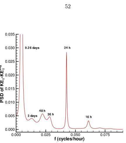
As a second step, we identify the main frequency components of the real-time DLE peak curve over the shortened time interval [t0, t−T]. Shown in Fig. 4.9, the power

spectrum density of the real-time DLE peak curve highlights seven dominant frequency components, with the importance of each frequency determined by the area under the corresponding spike in the spectrum. Surprisingly, the most influential component is not the tidal oscillation (with a period of 24 hours) or any of its harmonics, but rather a component with a period of 8.6 days.

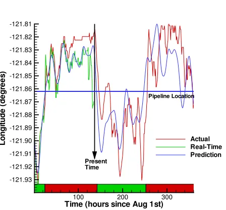
To complete our prediction procedure, we now use all the dominant Fourier modes of Fig. 4.9 to generate a prediction for the DLE peak location along the axis of the pipeline. The amplitudes and phases of the prediction curve are determined by minimizing the norm of the difference (i.e., the integral of the squared difference) between predicted and real-time DLE values. Fig. 4.10 shows the predicted DLE peak location together with the actual and the real-time locations. Note how faithfully the predicted curve reproduces the main features of the actual DLE peak oscillation.

Figure 4.9: Power spectrum density of the real-time DLE peak oscillations shown in Fig. 4.7. The spikes at 48 hours and 4 days indicate harmonics associated with the 24-hour tidal oscillation. The importance of each frequency is proportional to the area below the corresponding spike.

5 hours and 110 hours from the present time,t= 135 hours, will cause most of the pollution to exit Monterey Bay without recirculation. Pollution released between 160 and 175 hours will not leave the bay immediately due to a short-lived excursion of the actual DLE peak curve into longitudes on the coastal side of the pipe outlet (see Fig. 4.10). However, assuming a constant rate of pollution release throughout the interval [140h,250h], one finds that recirculating contaminants constitute less than 15% of the total amount of contaminants released.

Figure 4.10: Actual, real-time, and predicted DLE peak location along the ax is of the pipeline. The horizontal line marks the location of the outlet of the pipe. The colorbar indicates the periods of desirable releases (green) and the periods to avoid (red).