Exploring Approaches to Discriminating among Near Synonyms

Exploring approaches to discriminating among near-synonyms

Mary Gardiner

Centre for Language Technology Macquarie University [email protected]

Mark Dras

Centre for Language Technology Macquarie University [email protected]

Abstract

Near-synonyms are words that mean ap-proximately the same thing, and which tend to be assigned to the same leaf in ontolo-gies such as WordNet. However, they can differ from each other subtly in both mean-ing and usage—consider the pair of near-synonymsfrugalandstingy—and therefore choosing the appropriate near-synonym for a given context is not a trivial problem.

Initial work by Edmonds (1997) suggested that corpus statistics methods would not be particularly effective, and led to subsequent work adopting methods based on specific lexical resources. In earlier work (Gardiner and Dras, 2007) we discussed the hypoth-esis that some kind of corpus statistics ap-proach may still be effective in some situa-tions, particularly if the near-synonyms dif-fer in sentiment from each other, and we presented some preliminary confirmation of the truth of this hypothesis. This suggests that problems involving this type of near-synonym may be particularly amenable to corpus statistics methods.

In this paper we investigate whether this re-sult extends to a different corpus statistics method and in addition we analyse the re-sults with respect to a possible confound-ing factor discussed in the previous work: the skewness of the sets of near synonyms. Our results show that the relationship be-tween success in prediction and the nature of the near-synonyms is method dependent and that skewness is a more significant factor.

1 Introduction

Choosing an appropriate word or phrase from among candidate near-synonyms or paraphrases is a significant language generation problem since even though near-synonyms and paraphrases are close in meaning, they differ in connotation and denotation in ways that may be significant to the desired effect of the generation output: for example, word choice can change a sentence from advice to admonish-ment. Particular applications that have been cited as having a use for modules which make effective word and phrase choices among closely related options are summarisation and rewriting (Barzilay and Lee, 2003). Inkpen and Hirst (2006) extended the genera-tion system HALogen (Langkilde and Knight, 1998; Langkilde, 2000) to include such a module.

We discuss a particular aspect of choice between closely related words and phrases: choice between words when there is any difference in meaning or at-titude. Typical examples arefrugalandstingy; slen-derandskinny; anderrorandblunder.

In this paper, as in Gardiner and Dras (2007), we explore whether corpus statistics methods have promise in discriminating between near-synonyms with attitude differences, particularly compared to near-synonyms that do not differ in attitude. In our work, we used the work of (Edmonds, 1997), the first to attempt to distinguish among near-synonyms, adopting a corpus statistics approach. Based on that work, we found that there was a significant difference in attitudinal versus non-attitudinal near-synonyms. However, the Edmonds algorithm pro-duced on the whole poor results, only a little above the given baseline, if at all. According to (Inkpen, 2007), the poor results were due to the way the

gorithm handled data sparseness; she consequently presented an alternative algorithm with much bet-ter results. We also found that attitudinal versus non-attitudinal near-synonyms differed significantly in their baselines as a consequence of skewness of synset distribution, complicating analysis.

In this paper then we develop an algorithm based on that of Inkpen, and use a far larger data set and a methodology suited to large data sets, to see whether this alternative method will support our pre-vious findings. In addition we analyse results with regard to a measure of synset skewness. In Sec-tion 2 we outline the near-synonym task descrip-tion; in Section 3 we present our method based on Inkpen; in Section 5 we present out method based on Inkpen, and our experimental method using it; in Section 4 we evaluate its effectiveness in compari-son with Inkpen’s own method; in Section 5 we test our hypothesis, present our results and discuss them; and in Section 6 we conclude.

2 Task Description

Our experiment tests a system’s ability to fill a gap in a sentence from a given set of near-synonyms. This problem was first described by Edmonds (1997). Edmonds describes an experiment that he designed to test whether or not co-occurrence statistics are sufficient to predict which word in a set of near-synonyms fills alexical gap. He gives this example of asking the system to choose which oferror, mis-takeoroversightfits into the gap in this sentence:

(1) However, such a move also of cutting deeply into U.S. economic growth, which is why some economists think it would be a

big .

Performance on the task is measured by compar-ing system performance against real word choices: that is, sentences such as example 1 are drawn from real text, a word is removed, and the system is asked to choose between that word and all of its near-synonyms as candidates to fill the gap.

3 An approximation to Inkpen’s solution to the near-synonym choice problem

We know of two descriptions of algorithms used to choose between near-synonyms based upon

con-text: that described by Edmonds (1997) and that de-scribed by Inkpen (2007).

In our previous work we used Edmonds’ method for discriminating between near-synonyms as a ba-sis for comparing whether near-synonyms that differ in attitude in predictability from near-synonyms that do not. The more recent work by Inkpen is a more robust and reliable approach to the same problem, and therefore in this paper we develop a methodol-ogy based closely on that of Inkpen, using a differ-ent style of training corpus, in order to test whether the differences between the performance of near-synonyms that differ in sentiment and those that do not persists on the better performing method.

Edmonds’ and Inkpen’s approaches to near-synonym prediction have the same underlying hy-pothesis: that the choice between near-synonyms can be predicted to an extent from the words im-mediately surrounding the gap. Returning to exam-ple 1, their approaches use words around the gap, eg

big, to predict which oferror, mistakeoroversight

would be used. They do this using some measure of how oftenbig, and other words surrounding the gap, is used in contexts where each oferror,mistakeand

oversightare used. Edmonds uses every word in the sentence containing the gap, whereas Inkpen uses a generally smaller window of words surrounding the gap.

In this section we briefly describe Edmonds’ ap-proach to discriminating between near-synonyms in Section 3.1 and describe Inkpen’s approach in more detail in Section 3.2. We then describe our adapta-tion of Inkpen’s approach in Secadapta-tion 3.3.

3.1 Edmonds’ approach

In Edmonds’ approach to the word choice problem, the suitability of any candidate wordcfor a sentence

S can be approximated as a score(c, S) of suitabil-ity, and where score(c,S) is a sum of the association between the candidatecand every other wordwin the sentence.

score(c, S) = X w∈S

sig(c, w)

(2)

a wordw0and the same wordw0withw. Edmonds’ t-scores were computed using co-occurrence counts in the 1989 Wall Street Journal, and the performance did not improve greatly over a baseline of choosing the most frequent word in the synset to fill all gaps.

3.2 Inkpen’s approach

In Inkpen’s method, the suitability of candidatecfor a given gap is approximated slightly differently: the entire sentence is not used to measure the suitability of the word. Instead, a certain sized window of k

words either side of the gap is used. For example, if

k= 3, the word missing from the sentence in exam-ple 3 is predicted using only the six words shown in example 4.

(3) Visitors to Istanbul often sense a second, layer beneath the city’s tangible beauty.

(4) sense a second, layer beneath the

Given a text fragment f consisting of

2k words, k words either side of a gap g

(w1, w2, . . . , wk, g, wk+1, . . . , w2k), the

suit-abilitys(c, g) of any given candidate wordc to fill the gapgis given by:

s(c, g) = k

X

j=1

PMI(c, wj) + 2k

X

j=k+1

PMI(wj, c)

(5)

PMI(x, y) is the pointwise mutual information score of two wordsxandy, and is given by (Church and Hanks, 1991):

PMI(x, y) = log₂ C(x, y)·N C(x)·C(y)

(6)

C(x), C(y) and C(x, y) are estimated using to-ken counts in a corpus: C(x, y) is the number of times thatx and y are found together, C(x) is the total number of occurrences ofx in the corpus and

C(y)the total number of occurrences ofyin the cor-pus.N is the total number of words in the text.

Inkpen estimated C(x), C(y) and C(x, y) by issuing queries to the Waterloo MultiText Sys-tem (Clarke and Terra, 2003). She definedC(x, y)

the number of times wherexis followed byywithin a certainquery frameof lengthqwithin a corpus, so

that, for example, ifq = 3, example 7 would count as a co-occurrence offresh and mango, but exam-ple 8 would not:

(7) He likesfreshcoldmango.

(8) I like fresh fruits in general, particularly

mango.

She also experimented with document counts where C(x) is the number of documents that x is found in andC(x, y)is the number of documents in which bothxandy are found, called PMI-IR (Tur-ney, 2001); but found that this method did not per-form as well, although the difference was not statis-tically significant.

Inkpen’s method outperformed both the baseline and Edmonds’ method by 22 and 10 percentage points respectively.

3.3 Our variation of Inkpen’s approach

Our variation on Inkpen’s approach is designed to estimate PMI(x, y), the pointwise mutual informa-tion of words x and y, using the Web 1T 5-gram corpus Version 1 (Brants and Franz, 2006).

Web 1T contains n-gram frequency counts, up to and including 5-grams, as they occur in a trillion words of World Wide Web text. There is no con-text information beyond the n-gram boundaries. Ex-amples of a 3-gram and a 5-gram and their respec-tive counts from Web 1T are shown in examples 9 and 10:

(9) means official and 41

(10) Valley National Park 1948 Art

51

These n-gram counts allow us to estimateC(x, y)

for a given window width k by summing the Web 1T counts ofk-grams in which wordsxandyoccur andxis followed byy.

Counts are computed using a an especially de-veloped version of the Web 1T processing software “Get 1T”1 originally described in Hawker (2007) and detailed in Hawker et. al (2007). The Get 1T software allows n-gram queries of the form in the following examples, where<*>is a wildcard which

1

will match any token in that place in the n-gram. In order to find the number of n-grams withfresh and

mangowe need to construct three queries:

(11) <*> fresh mango

(12) fresh <*> mango

(13) fresh mango <*>

However, in order to findfreshandmangowithin 4 grams we need multiple wildcards as in exam-ple 14, and added the embedded query hashing func-tionality described in Hawker et. al (2007).

(14) fresh <*> <*> mango

Queries are matched case-insensitively, but no stemming takes place, and there is no deeper anal-ysis (such as part of speech matching).

This gives us the following methodology for a given lexical gapg and a window ofkwords either side of the gap:

1. for every candidate near-synonymc:

(a) for every word wi in the set of words

proceeding the gap,w1, . . . , wk, calculate

PMI(wi, c)as in equation 6, given counts

for C(wi), C(c) and C(wi, c) from Web

1T2

(b) for every wordwj in the set of words

fol-lowing the gap, wk+1, . . . , w2k, calculate

PMI(c, wj)as in equation 6, given counts

for C(c), C(wj)andC(c, wj) from Web

1T

(c) compute the suitability score s(c, g) of candidatecas given by equation 5

2. select the candidate near-synonym with the highest suitability score for the gap where a sin-gle such candidate exists

3. where there is no single candidate with a high-est suitability score, select the most frequent candidate for the gap (that is, fall back to the baseline described in Section 3.4)3

2

The result of equation 6 is undefined when any ofC(x) = 0,C(y) = 0orC(x, y) = 0hold, that is, xoryor at least one n-gram containingx andy cannot be found in the Web 1T counts. For the purpose of computings(c, g), we define PMI(x, y) = 0whenC(x) = 0,C(y) = 0orC(x, y) = 0, so that it has no influence on the scores(c, g)given by equation 5.

3

Typically, in this case, all candidates have scored 0.

Since Web 1T contains 5-gram counts, we can use query frame sizes fromq = 1(wordsx andymust be adjacent, that is, occur in the 2-gram counts) to

q= 4.

3.4 Baseline method

The baseline method that our method is compared to uses the most frequent word from a given synset as the chosen candidate for any gap requiring a mem-ber of that synset. Frequency is measured using fre-quency counts of the combined part of speech and word token in the 1989 Wall Street Journal.

4 Effectiveness of the approximation to Inkpen’s method

In this section we compare our approximation of Inkpen’s method described in Section 3.3 with her method described in Section 3.2. This will allow us to determine whether our approximation is effective enough to allow us to compare attitudinal and non-attitudinal near-synonyms.

4.1 Test sets

In order to compare the two methods, we use five sets of near-synonyms, also used as test sets by both Edmonds and Inkpen:

• the adjectivesdifficult,hardandtough;

• the nounserror,mistakeandoversight;

• the nounsjob,taskandduty;

• the nouns responsibility, burden, obligation

andcommitment; and

• the nounsmaterial,stuffandsubstance.

Inkpen compared her method to Edmonds’ using these five sets and two more, both sets of verbs, which we have not tested on, as our attitudinal and non-attitudinal data does not included annotated verbs. We are therefore interested in the predictive power of our method compared to Inkpen’s and Ed-mond’s on adjectives and nouns.

4.2 Test contexts

a source of test sentences.4 Where ever one of the words in a test set is found, it is removed from the context in which it occurs to generate a gap for the algorithm to fill.

So, for example, when sentence 15 is found in the test data, the worderroris removed from it and the system is asked to predict which oferror,mistakeor

oversightfills the gap at 16:

(15) . . .his adversarys’ characterization of that minor sideshow as somehow a colossal er-roron the order of a World War. . ..

(16) a colossal on the

4.3 Parameter settings

Recall from Section 3.2 these two parameters used by Inkpen: kandq.

Parameterkis the size of the ‘window’ of context on either side of a lexical gap in the test set: the

kwords on either side of a gap are used to predict which of the candidate words best fills the gap.

Parameterqis the query size used when querying

the corpusto find out how often wordsxandyoccur together in order to compute the value ofC(x, y). In order to be counted as occurring together, x and y

must occur within a window of length at mostq. Inkpen found, using Edmonds’ near-synonym set

difficultandhardas a development set, that results are best for a small window (k∈ {1,2}) but that the query frame had to be somewhat longer to get the best results. Her results were reported usingk = 2

andq = 5, chosen via tuning on the development set.

We have retained the settingk = 2and explored results where q = 2 and q = 4: due to Web 1T containing 5-grams but no higher order n-grams we cannot measure the frequency of two words occur-ring together with any more than three intervening words, soq= 4is the highest valueqcan have.

4.4 Results and Discussion

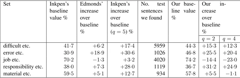
Table 1 shows the performance of Edmonds’ method and Inkpen’s method as given in Inkpen (2007)5and

4

All references to the Wall Street Journal data used in this paper refer to Charniak et. al (2000).

5

Inkpen actually gives two methods, one using PMI esti-mates from document counts, one using PMI estiesti-mates using word counts. Here we are discussing her word count method and use those values in our table.

our modified method on each of the test sets de-scribed in Section 4.1. Note that Inkpen reports dif-ferent baseline results from us—we have not been able to reproduce her baselines. This may be due to choosing different part of speech tags: we simply usedJJfor adjectives andNNfor nouns.

Inkpen’s improvements for the test synsets given in Section 4.1 were between +3.2% and 30.6%. Our performance is roughly comparable, with improve-ments as high as 31.2%. Further, we tend to improve especially largely over the baseline where Inkpen also does so: on the two setserroretc and responsi-bilityetc..

The major anomaly when compared to Inkpen’s performance is the set job, task and duty, where our method performs very badly compared to both Edmonds’ and Inkpen’s methods and the baseline (which perform similarly). We also perform under both methods onmaterial, stuff and substance, al-though not as dramatically.

Overall, the fact that we tend to improve over Ed-monds where Inkpen also does so suggests that our algorithm based on Inkpen’s takes advantage of the same aspects as hers to gain improvements over Ed-monds, and thus that the method is a good candidate for use in our main experiment.

5 Comparing attitudinal and non-attitudinal synsets

Having determined in Section 4 that our modified version of Inkpen’s method performs as a passable approximation of hers, and particularly that where her method improved dramatically over the baseline and Edmonds’ method that ours improves likewise, we then tested our central hypothesis: that attitu-dinal synsets respond better to statistical prediction techniques than non-attitudinal synsets.

5.1 Test set

In order to test our hypothesis, we use synsets di-vided into near-synonym sets that differ in attitudi-nal and sets that do not.

This test set is drawn from our set of annotated

Set Inkpen’s baseline value %

Edmonds’ increase over baseline %

Inkpen’s increase over baseline (q = 5) %

No. test sentences we found

Our base-line value %

Our

in-crease over baseline %

q = 2 q = 4

difficult etc. 41·7 +6·2 +17·4 5959 44·3 +15·3 +12·3

error etc. 30·9 +18·9 +30·6 1026 46·8 +25·5 +20·4

job etc. 70·2 −1·3 +3·2 4020 74·2 −14·4 −23·0

responsibility etc. 38·0 +7·3 +28·0 1119 36·7 +31·2 +24·9

material etc. 59·5 +5·1 +12·7 934 57·8 +5·5 −1·1

Table 1: Performance of Inkpen’s test sentences on Edmond’s method, Inkpen’s method and our method (k= 2)

Street Journal. The synsets were annotated as at-titudinal and non-attitudinal by the authors of this paper. Synsets were chosen where both annotators are certain of their label, and where both annotators have the same label. This results in 60 synsets in to-tal: 8 where the annotators agreed that there was def-initely an attitude difference between words in the synset, and 52 where the annotators agreed that there were definitely not attitude differences between the words in the synset.

An example of a synset agreed to have attitudinal differences was:

(17) bad,insecure,risky,high-risk,speculative

An example of synsets agreed to not have attitu-dinal differences was:

(18) sphere,domain,area,orbit,field,arena

The synsets are not used in their entirety, due to the differences in the number of words in each synset (compare {violence, force} with two members to

{arduous, backbreaking, grueling, gruelling, hard,

heavy, laborious, punishing, toilsome} with nine, for example). Instead, a certain numbernof words are selected from each synset (where n ∈ {3,4}) based on the frequency count in the 1989 Wall Street Journal corpus. For examplehard,heavy,gruelling

and punishing are the four most frequent words in the{arduous, backbreaking,grueling,gruelling,

hard,heavy,laborious,punishing,toilsome}synset, so whenn= 4those four words would be selected. When the synset’s length is less than or equal ton,

for example whenn= 4but the synset is{violence,

force}, the entire synset is used.

These test sets are referred to astop3(synsets re-duced to 3 or less members) andtop4 (synsets re-duced to 4 or less members).

5.2 Test contexts

Exactly as in Section 4.2, our lexical gaps and their surrounding contexts are drawn from sentences in the 1987 Wall Street Journal containing one of the words in the test synsets.

5.3 Parameter settings

As described in Sections 3.2 and 4.3, there are two parameters that can be varied regarding the context around a lexical gap (k), and the nearness of two wordsxandy in the corpus in order for them to be considered to occur together (q).

As per Inkpen’s results on her development set, and as in Section 4 we use the setting k = 2and varyqsuch thatq = 2on some test runs andq = 4

on others. We cannot test with Inkpen’s suggested

q= 5, as that would require 6-grams.

5.4 Results and Discussion

The overall performance of our method on our sets of attitudinal and non-attitudinal near-synonyms is shown in Table 2.

We did four test runs in total, two each on sets

Contexts containing a test word

Baseline correctness (%) q Our method’s correctness (%)

Synsets Att. Non-att. Att. Non-att. Att. Non-att.

top3 45953 353155 59·52 69·71 2 59·51 69·95

4 56·93 69·96

top4 48515 357290 56·37 68·91 2 52·26 67·60

4 50·82 67·59

Table 2: Performance of the baseline and our method on all test sentences (k= 2)

Improvement over

baseline

Number of synsets

Att. Non-att. Total

≥+20% 0 16 16

≥+10% and<+20% 1 7 8

≥+5% and<+1% 2 2 4

>-5% and<-5% 2 10 12

≤-5% and>-10% 0 6 6

≤-10% and>-20% 1 3 4

≤-20% 1 8 9

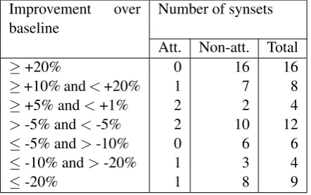
Table 3: Distribution of improvements on baseline fortop3,k= 2,q= 2

As in our previous paper (Gardiner and Dras, 2007), the baselines behave noticeably differently for attitudinal and non-attitudinal synsets. Calculat-ing thez-statistic as is standard for comparing two proportions (Moore and McCabe, 2003) we find that the difference between the pair of attitudinal and non-attitudinal results for each test are all statisti-cally significant (p < 0.01). Thus, again, it is dif-ficult from the data in Table 2 alone to determine whether the better performance of non-attitudinal synsets is due to the higher baseline performance for those same synsets.

There are two major aspects of this result requir-ing further investigation. The first is that our method performs very similarly to the baseline according to these aggregate numbers, which wasn’t anticipated based on the results in Section 4, which showed that on a limited set of synsets our method performed well above the baseline, although not as well as Inkpen’s original method.

Secondly, inspection of individual synsets and their performance reveals that this aggregate is not representative of the performance as a whole: it is

simply an average of approximately equal numbers of good and bad predictions by our method. Table 3 shows that for one test run (top3,k= 2,q= 2) there were a number of synsets on which our method per-formed very well with an improvement of more than 20 percentage points over the baseline but also a sub-stantial number where it performed very badly, los-ing more than 20 percentage points from the base-line.

In our previous work we expressed a suspicion that the success of Edmonds’ prediction method might be being influenced by the evenness of dis-tribution of frequencies within a synset. That is, if a synset contains a very dominant member (which will cause the baseline to perform well) then the Ed-monds method may perform worse against the base-line than it would for a synset in which the word choices were distributed fairly evenly among the members of the set.

Given the results of the test runs shown in Table 2, and the wide distribution of prediction successes shown in Table 3, we decided to test this hypothe-sis that the distribution of words in the synsets influ-ence the performance of prediction methods that use context. This is described in Section 5.4.1.

5.4.1 Entropy analysis

In this section, we describe an analysis of the re-sults in Section 5.4 in terms of whether the balance of frequencies among words in the synset contribute to the quality of our prediction result.

Test set q Category Entropy

top3 2 −0·11 0·41∗

top3 4 −0·10 0·36∗

top4 2 −0·17∗ 0·38∗

top4 4 −0·15∗ 0·34∗

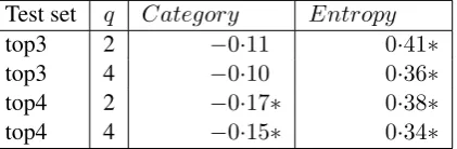
Table 4: Regression co-efficients between inde-pendent variables synset category and synset en-tropy, and dependent variable prediction improve-ment over baseline (statistically significant results

p <0.05marked *)

of total uses of the synset that each particular word represents. A synset in which frequencies are rea-sonably evenly distributed has high information en-tropy and a synset in which one or more words are very frequent as a proportion of use of that synset as a whole have low entropy.

We then carried out multiple regression analysis using the category of the synset (attitudinal or not attitudinal, coded as 1 and 0 for this analysis) and the entropy of the synset’s members’ frequencies as our two independent variables; this allows us to sep-arate out the two effects of synset skewness and at-titudinality. Regression co-efficients are shown in Table 4.

Table 4 shows that in general, performance is neg-atively correlated with both category but positively with entropy, although the correlation with category is not always significant. The positive relationship with entropy confirms our suspicion in Gardiner and Dras (2007) that statistical techniques perform bet-ter when the synset does not have a highly dominant member. The negative correlation with category im-plies that the reverse of our main hypothesis holds: that our statistical method works better for predict-ing the use of non-attitudinal near-synonyms.

There are two questions that arise from the result that our Inkpen-based method gives a different result from the Edmonds-based one.

First, is our approximation to Inkpen’s method in-herently faulty or can it be improved in some way? We know from Section 4 that it tends to perform well where her method performs well. An obvious second test is to compare our results to another test described in Inkpen (2007) which used a larger set of near-synonyms and tested the predictive power

using the British National Corpus as a source of test contexts. This test will test our system’s per-formance in genres quite different from news-wire text, and allow us to make a further comparison with Inkpen’s method.

Second, why do we perform significantly better for near-synonyms without attitude difference? One possible explanation that we intend to explore is that attitude differences are predicted by attitude differ-ences exhibited in a very large context; perhaps an entire document or section thereof. Sentiment anal-ysis techniques may be able to be used to detect the attitude bearing parts of a document and these may serve as more useful features for predicting attitudi-nal word choice than surrounding words.

6 Conclusion and Future Work

In this paper we have developed a modification to Inkpen’s method of making a near-synonym choice that on a set of her test data performs reasonably promisingly; however, when tested on a larger set of near-synonyms on average it does not perform very differently to the baseline. We have also shown that, contrary to our hypothesis that near-synonyms with attitude differences would perform better us-ing statistical methods, on this method the near-synonyms without attitude differences are predicted better when there’s a difference in predictive power. Ultimately, we plan to develop a system that will acquire and predict usage of attitudinal near-synonyms, drawing on statistical methods and meth-ods from sentiment analysis. In order to achieve this we will need a comprehensive understanding of why this method’s performance was not adequate for the task.

Acknowledgements

Thank you to: Diana Inkpen for sending us a copy of Inkpen (2007) while it was under review; and Tobias Hawker for providing a copy of his Web 1T process-ing software, Get 1T, before its public release.

References

Regina Barzilay and Lillian Lee. 2003. Learning to

paraphrase: An unsupervised approach using

multiple-sequence alignment. InHLT-NAACL 2003: Main

Pro-ceedings, pages 16–23.

Thorsten Brants and Alex Franz. 2006. Web 1T 5-gram

Version 1. http://www.ldc.upenn.edu/

Catalog/CatalogEntry.jsp?catalogId= LDC2006T13.

Eugene Charniak, Don Blaheta, Niyu Ge, Keith Hall,

John Hale, , and Mark Johnson. 2000. BLLIP

1987-89 WSJ Corpus Release 1. http://www.

ldc.upenn.edu/Catalog/CatalogEntry. jsp?catalogId=LDC2000T43.

Kenneth Church and Patrick Hanks. 1991. Word asso-ciation norms and mutual information, lexicography.

Computational Linguistics, 16(1):22–29.

Charles L. A. Clarke and Egidio L. Terra. 2003. Passage retrieval vs. document retrieval for factoid question

an-swering. In Proceedings of the 26th Annual

Interna-tional ACM SIGIR Conference on Research and De-velopment in Information Retrieval, pages 427–428, Toronto, Canada.

Philip Edmonds. 1997. Choosing the word most typical in context using a lexical co-occurrence network. In

Proceedings of the 35th Annual Meeting of the Associ-ation for ComputAssoci-ational Linguistics and the 8th Con-ference of the European Chapter of the Association for Computational Linguistics, pages 507–509, July.

Christiane Fellbaum, editor. 1998. WordNet: An

Elec-tronic Lexical Database. The MIT Press, May.

Mary Gardiner and Mark Dras. 2007. Corpus statistics approaches to discriminating among near-synonyms. In Proceedings of the 10th Conference of the Pacific Association for Computational Linguistics (PACLING 2007), pages 31–39, Melbourne, Australia, September.

Tobias Hawker, Mary Gardiner, and Andrew Bennetts. 2007. Practical queries of a massive n-gram database. InProceedings of the Australasian Language Technol-ogy Workshop 2007 (ALTW 2007), Melbourne, Aus-tralia. To appear.

Tobias Hawker. 2007. USYD: WSD and lexical

substi-tution using the Web 1T corpus. In Proceedings of

SemEval-2007: the 4th International Workshop on Se-mantic Evaluations, Prague, Czech Republic.

Diana Inkpen and Graeme Hirst. 2006. Building and using a lexical knowledge-base of near-synonym

dif-ferences. Computational Linguistics, 32(2):223–262,

June.

Diana Inkpen. 2007. A statistical model of

near-synonym choice. ACM Transactions of Speech and

Language Processing, 4(1):1–17, January.

Irene Langkilde and Kevin Knight. 1998. The practical value of N-grams in generation. InProceedings of the 9th International Natural Language Generation

Work-shop, pages 248–255, Niagra-on-the-Lake, Canada.

Irene Langkilde. 2000. Forest-based statistical sentence

generation. In Proceedings of the 1st Conference of

the North American Chapter of the Association for Computational Linguistics and the 6th Conference on Applied Natural Language Processing (NAACL-ANLP 2000), pages 170–177, Seattle, USA.

David S. Moore and George P. McCabe. 2003.

Introduc-tion to the Practice of Statistics. W. H. Freeman and Company, 4 edition.

Claude E. Shannon. 1948. A mathematical theory

of communication. Bell System Technical Journal,

27:379–423 and 623–656, July and October.

Peter Turney. 2001. Mining the web for synonyms:

PMI-IR versus LSA on TOEFL. In Proceedings of