Grounding Word Meanings in Sensor Data:
Dealing with Referential Uncertainty
Tim Oates
Department of Computer Science and Electrical Engineering
University of Maryland Baltimore County
1000 Hilltop Circle
Baltimore, MD 21250
[email protected]
Abstract
We consider the problem of how the mean-ings of words can be grounded in sensor data. A probabilistic representation for the mean-ings of words is defined, a method for recov-ering meanings from observational information about word use in the face of referential uncer-tainty is described, and empirical results with real utterances and robot sensor data are pre-sented.
1
Introduction
We are interested in how robots might learn language given qualitatively the same inputs available to children -natural language utterances paired with sensory access to the environment. This paper focuses on the sub-problem of learning word meanings. Suppose a robot has acquired a set of sound patterns that may or may not correspond to words. How is it possible to separate the words from the non-words, and to learn the meanings of the words?
We assume the robot’s sensory access to its environ-ment is through a collection of primitive sensors orga-nized into sensor groups, where each sensor group is a set of related sensors. For example, the sensor group
might return a single value representing the mean grayscale intensity of a set of pixels corresponding to an object in the visual field. The sensor group
might return two values representing the height and width of the bounding box around the object.
Learning the meanings of words requires a represen-tation for meaning. We use a represenrepresen-tation that we call a conditional probability field (CPF), which is a type of scalar field. A scalar field is a map of the following form:
The mapping assigns to each vector
a scalar value
. A conditional probability field assigns to each ,
which corresponds to a point in an -dimensional sen-sor group, a conditional probability of the form
E , where E denotes the occurrence of some event. Let
E
denote the CPF defined over sensor group for eventE.
The semantics of a CPF clearly depend on the nature ofE. Two events that will be of particular importance in learning the meanings of words are:
utter-W- the event that word is uttered, per-haps as part of an utterance that refers to some fea-ture of the world denoted by
hear-W- the event that word is heard
The corresponding conditional probability fields are:
utter-W
- the probability that word will be uttered by a competent speaker of the language to denote the feature of the physical world that is currently sensing (i.e. that results in the current value of )
hear-W
- the probability that word will be heard given that is observed
In this framework, the meaning of word is simply
utter-W
. The last plot in figure 3 shows a CPF defined over that might represent the meaning of the word “gray”. Grayscale intensities near 128 will be called gray with probability almost one, whereas intensities near 0 and 255 will never be called gray. Rather, they are “black” and “white” respectively.
Learning the denotation of involves determining the identity of and then recoveringutter-W
. The learner does not have direct access toutter-W
. Rather, the learner must gain information about
utter-W
indirectly, by noticing the sensory con-texts in which is used and those in which it is not, i.e. viahear-W
This problem is difficult due to referential uncertainty. Even if the utterances the learner hears are true state-ments about aspects of its environment that are percep-tually available, there are are usually many aspects of the environment that might be a given word’s referent. This is Quine’s “gavagai” problem (Quine, 1960). The algo-rithm described in this paper solves a restricted version of the gavagai problem, one in which the denotation of a word must be representable as a CPF defined over one of a set of pre-defined sensor groups.
2
A Simplified Learning Problem
Rather than starting with the full complexity of the prob-lem facing the learner, consider the following highly sim-plified version. Suppose an agent with a single sensor group, , lives in a world with a single object, , that periodically changes color. Each time the color changes, a one word utterance is generated describing the new color, which is one of “black”, “white” or “gray”.
In this scenario there is no need to identify because there is only one possibility. Also, each time a word is uttered there is perfect information about its denotation; it is the current value produced by
. (The nota-tion
indicates the value recorded by sensor group when it is applied to object . This assumes an ability to individuate objects in the environment.) Therefore, the probability that a native speaker of our simple language will utter to refer to is the same as the probability of hearing given . This fact makes it possible to recover the form of the CPF for each of the three words by notic-ing which values of
co-occur with the words and applying Bayes’ rule as follows:
utter-W
hear-W
hear-W
hear-W
hear-W
The maximum-likelihood estimate of the quantity
hear-W is simply the number of utterances contain-ing divided by the total number of utterances. The quantities
and
hear-W can be estimated using a number of standard techniques. We use kernel density estimators with (multivariate) Gaussian kernels to esti-mate probability densities such as these.
The simplified version of the word-learning problem presented in this section can be made more realistic, and thus more complex, by increasing either the num-ber of objects in the environment or the numnum-ber of sensor groups available to the agent. Section 3 explores the for-mer, and section 4 explores the latter.
3
Multiple Objects
When there is no ambiguity about the referent of a word, it is possible to recover the conditional probability field that represents the word’s denotational meaning by pas-sive observation of the contexts in which it is used. Un-fortunately, referential ambiguity is a feature of natural languages that we contend with on a daily basis. This ambiguity appears to be at its most extreme for young children acquiring their first language who must deter-mine for each newly identified word the referent of the word from the infinitely many aspects of their environ-ment that are perceptually available.
Consider what happens when we add a second object,
, to our example domain. If both objects change color at exactly the same time, though not necessarily to the same color, the learner has no way of knowing whether an utterance refers to the value produced by
or
. In the absence of any exogenous information about the referent, the best the learner can do is make a guess, which will be right only of the time. As the number of objects in the environment increases, this percentage decreases.
Referential ambiguity can also take the form of un-certainty about the sensor group to which a word refers. Given two objects, and , and two sensor groups, and , a word can refer to any of the following:
,
,
,
. In this section we make the un-realistic assumption that the learner has a priori knowl-edge about the sensor group to which a word refers. This assumption will be relaxed in the following section.
Intuitively, referential ambiguity clouds the relation-ship between the denotational meaning of a word and the observable manifestations of its meaning, i.e. the contexts in which the word is used. As we will now demonstrate, it is possible to make the nature of this clouding precise, leading to an understanding of the impact of referential ambiguity on learnability.
Suppose an agent hears an utterance containing word while its attention is focused on the output of sensor group . (Recall that in this section we are mak-ing the assumption that the agent knows that refers to .) Why might contain ? There are two mutu-ally exclusive and exhaustive cases: is (at least in part) about , and is chosen to denote the current value pro-duced by ; is not about , and contains despite this fact. The latter case might occur if, for example, has multiple meanings and the utterance uses one of the meanings of that does not denote a value produced by
.
Let
denote the fact that is (at least in part) about , and let
hear-W (1) utter-W (2)
Figure 1: A derivation of the relationship betweenhear-W
andutter-W .
produced by can be expressed via equation 1 in figure 1. Equation 1 is a more formal, probabilistic statement of the conditions given above under which will contain
. It can be simplified as shown in the remainder of the figure.
The first step in transforming equation 1 into equation 2 is to apply the fact that
. The resulting joint probability is the probability of a conjunction of terms that contains both
and
, and is therefore 0 and can be dropped. The remaining two terms are then rewritten using Bayes’ rule. Finally, three substitutions are made:
utter-W Simplification then leads directly to equation 2.
Before discussing the implications of equation 2, con-sider the import of and . The probability that is about (i.e. ) is the probability that the speaker and the hearer are attending to the same sensory information. When
, there is perfect shared attention, and the speaker always refers to those aspects of the physical environment to which the hearer is currently attending. When , there is never shared attention, and the speaker always refers to aspects of the environment other than those to which the hearer is currently attending.
The probability that contains even when is not about (i.e. ) is the probability that will be used to refer to some feature of the environment other than that measured by . There are two reasons why might occur in a sentence that does not refer to :
is polysemous and one of the meanings that does not refer to is used in the utterance
is used to refer to the value produced by for some object other than the one that is the hearer’s focus of attention (e.g.
rather than
)
Note that comes into play only when
, i.e. when there is less than perfect shared attention between the speaker and the hearer.
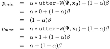
The most significant aspect of equation 2 is from the standpoint of learnability. In our original one-object, one-sensor world there was never any doubt as to the referent of a word, and it was therefore the case that
utter-W hear-W
. This equivalence becomes clear in equation 2 by setting
and simpli-fying. Because it is possible to computehear-W
from observable information via Bayes’ rule, it was pos-sible in that world to recoverutter-W
rather di-rectly. However, equation 2 tells us that even in the face of imperfect shared attention (i.e.
) and homonymy (i.e. ) it is the case thathear-W
is a linear transform ofutter-W
. Moreover, the values of and determine the precise nature of the transform.
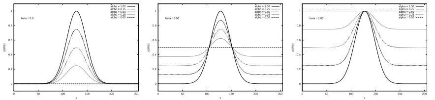
To get a better handle on the effects of and
on the manifestation of utter-W
through
hear-W
, consider figures 2 and 3. The last plot in figure 2 shows an example of a conditional prob-ability field utter-W
, which is also a plot of
hear-W
when
. Figures 2 and 3 demon-strate the effects of varying and onhear-W
. That is, the figures show how varying and affect the information aboututter-W
available to the learner.
Recall from equation 2 that the conditional probability that word will be heard given the current value pro-duced by is a linear function ofutter-W
which has slope and intercept
. When the slope is zero (i.e. ) the speaker and the hearer never focus on the same features of the environment, and the prob-ability of hearing is just the background probability of hearing , independent of the value of . When the slope is one (i.e.
figure 2, which contains plots ofhear-W
over a range of values of for various fixed values of .
Figure 2 makes it clear that decreasing preserves the overall shape of utter-W
as observed through
hear-W
, while squashing it to fit in a smaller range of values. Increasing diminishes the effect of , which is to offset the entire curve vertically. That is, the higher the level of shared attention between speaker and hearer, the less the impact of the background frequency of
on the observable manifestation ofutter-W
[image:4.612.330.522.190.276.2]
. Figure 3, which shows plots ofhear-W
given a range of values of for various fixed values of
, is another way of looking at the same data. The role of in squashing the observable manifestation of
utter-W
is apparent, as is the role of in ver-tically shifting the curves. Only when is there no information about the form ofutter-W
in the plot ofhear-W
.
What does all of this have to say about the impact of
and on the learnability of word meanings from sen-sory information about the contexts in which they are ut-tered? As we will demonstrate shortly, if the following expression is true for a given conditional probability field,
utter-W
, then it is possible to recover that CPF from observable data (i.e. fromhear-W
):
utter-W
utter-W
The claim is as follows. If there is both a value produced by that is always referred to as and a value that is never referred to as , one can recover the CPF that represents the denotational meaning of simply by ob-serving the contexts in which is used.
Intuitively, the above expression places two constraints on word meanings. First, for a word whose denotation is defined over sensor group , it must be the case that some value produced by is (almost) universally agreed to have no better descriptor than ; there is no other word in the language that is more suitable for denoting this value. Second, there must be some value produced by for which it is (almost) universally agreed that is not the best descriptor. It is not necessarily the case that
is the worst descriptor, only that some other word or words are better.
As equation 2 indicates, hear-W
is a linear transform ofutter-W
with slope and intercept
. If we know two points on the line defined by equation 2 we can determine its parameters, making it possible to reverse the transform and compute the value ofutter-W
given the value ofhear-W
. Because hear-W
is a linear transform of
utter-W
, any value of that minimizes (maxi-mizes) one minimizes (maxi(maxi-mizes) the other. Recall that conditional probability fields map from sensor vectors to probabilities, which must lie in the range [0, 1]. Under
the assumption thatutter-W
takes on the value at some point, such as when ,hear-W
must be at its minimum value at that point as well. Let that value be . Likewise, under the assumption that
utter-W
takes on the value
at some point, such as when
, hear-W
must be at its maxi-mum value at that point as well. Let that value be . These observations lead to the following system of two equations:
utter-W
utter-W
Solving these equations for and yields the following:
Recall that the goal of this exercise is to re-cover utter-W
from its observable manifesta-tion,hear-W
. This can finally be accomplished by substituting the values for and given above into equation 2 and solving forutter-W
as shown in figure 4.
That is, one can recover the CPF that represents the de-notational meaning of a word by simply scaling the range of conditional probabilities of the word given observa-tions so that it completely spans the interval
.
4
Multiple Sensor Groups
This section considers a still more complex version of the problem by allowing the learner to have more than one sensor group. Suppose an agent has two sensor groups, and , and that word refers to . The agent can observe the values produced by both sensor groups, note whether each value co-occurred with an utterance containing , compute bothhear-W
and hear-W
, and apply equation 2 to obtain
utter-W
andutter-W
. How is the agent to determine thatutter-W
represents the meaning of andutter-W
is garbage? The key insight is that if the meaning of is grounded in , there will be some values of for which it is more likely that will be uttered than for others, and thus there will be some values for which it is more likely that will be heard than others. Indeed, our ability to recoverutter-W
fromhear-W
is founded on the assumption that there is some value of
0 0.2 0.4 0.6 0.8 1
0 50 100 150 200 250
p(W|x)
x alpha = 0.00
beta = 1.00 beta = 0.75 beta = 0.50 beta = 0.25 beta = 0.00
0 0.2 0.4 0.6 0.8 1
0 50 100 150 200 250
p(W|x)
x alpha = 0.50
beta = 1.00 beta = 0.75 beta = 0.50 beta = 0.25 beta = 0.00
0 0.2 0.4 0.6 0.8 1
0 50 100 150 200 250
p(W|x)
x alpha = 1.00
beta = 1.00 beta = 0.75 beta = 0.50 beta = 0.25 beta = 0.00
Figure 2: The effects of onhear-W
for various values of .
0 0.2 0.4 0.6 0.8 1
0 50 100 150 200 250
p(W|x)
x beta = 0.0
alpha = 1.00 alpha = 0.75 alpha = 0.50 alpha = 0.25 alpha = 0.00
0 0.2 0.4 0.6 0.8 1
0 50 100 150 200 250
p(W|x)
x beta = 0.50
alpha = 1.00 alpha = 0.75 alpha = 0.50 alpha = 0.25 alpha = 0.00
0 0.2 0.4 0.6 0.8 1
0 50 100 150 200 250
p(W|x)
x beta = 1.00
[image:5.612.93.522.113.214.2]alpha = 1.00 alpha = 0.75 alpha = 0.50 alpha = 0.25 alpha = 0.00
Figure 3: The effects of onhear-W
for various values of .
hear-W
utter-W
utter-W
utter-W
utter-W
hear-W
(3)
[image:5.612.86.528.327.429.2]is zero and some other value for which that probabil-ity is one. This is not necessarily the case for the con-ditional probability of hearing given because the level of shared attention between the speaker and the learner, , influences the range of probabilities spanned byhear-W
, with smaller values of leading to smaller ranges.
Note that in our simple example with two sensor groups the speaker considers only the value of when determining whether to utter , and the learner considers only the value of when constructinghear-W
. Using the terminology and notation developed in section 3, there is no shared attention between the speaker and the learner with respect to and , and it is therefore the case that andhear-W
.
If the exact value ofhear-W
is known for all , an obviously unrealistic assumption, it is a simple matter to determine that utter-W
cannot rep-resent the meaning of by noting that it is constant. Ifutter-W
is not constant, then the speaker is more likely to utter for some values of than for others, and the meaning of is therefore grounded in
. As indicated by figure 2, the height of the bumps in the conditional probability field depend on , the level of shared attention, but if there are any bumps at all we know that the meaning of is grounded in the corresponding sensor group and we can recover the underlying condi-tional probability field. Under the assumption that the exact value ofhear-W
can be computed, an agent can identify the sensor group in which the denotation of a word is grounded by simply recoveringutter-W
for each of its sensor groups and looking for the one that is not constant.
In practice, the exact value ofhear-W
will not be known, and it must be estimated from a finite number of observations. That is, an estimate ofhear-W
will be used to compute an estimate ofutter-W
. Even if there is no association between and , and
utter-W
is therefore truly constant, an estimate of this conditional probability based on finitely many data will invariably not be constant. Therefore, the strategy of identifying relevant sensor groups by looking for bumpy conditional probability fields will not work.
The problem is that for any given word and sen-sor group , it is difficult to distinguish between cases in which and are unrelated and cases in which the meaning of is grounded in but shared attention is low. The solution to this problem has two parts, both of which will be described in detail shortly. First, the mutual information between occurrences of words and sensor values will be used as a measure of the degree to which hearing depends on the value produced by , and vice versa. Second, a non-parametric statistical test based on randomization testing will be used to convert
the real-valued mutual information into a binary decision as to whether or not the denotation of is grounded in
.
4.1 Mutual Information
Let
denote the mutual information between oc-currences of word and values produced by sensor group . The value of
is defined as follows:
hear-W
hear-W
hear-W
hear-W
hear-W
hear-W
Note that
is the mutual information between two different types of random variables, one discrete ( ) and one continuous ( ). In the expression above, the summation over the two possible values of , i.e.hear-Wand hear-W, is unpacked, yielding a sum of two integrals over the values of . Within each in-tegral the value of is held constant. Finally, recall that
is a vector with the same dimensionality as the sensor group from which it is drawn, so the integrals above are actually defined to range over all of the dimensions of the sensor group.
When
is zero, knowing whether is uttered provides no information about the value produced by , and vice versa. When
is large, knowing the value of one random variable leads to a large reduction in uncertainty about the value of the other. Larger val-ues of mutual information reflect tighter concentrations of the mass of the joint probability distribution and thus higher certainty on the part of the agent about both the circumstances in which it is appropriate to utter and the denotation of when it is uttered.
Although mutual information provides a measure of the degree to which and are dependent, to under-stand and generate utterances containing the agent must at some point make a decision as to whether or not its meaning is in fact grounded in . How is the agent to make this determination based on a single scalar value? The next section describes a way of converting scalar mutual information values into binary decisions as to whether a word’s meaning is grounded in a sen-sor group that avoids all of the potential pitfalls just de-scribed.
4.2 Randomization Testing
Given word , sensor group , and their mutual infor-mation
occurrences of and the values produced by are not independent?
The latter question is the form used in statistical hy-pothesis testing. In this case the null hyhy-pothesis, , would be that occurrences of and the values produced by are independent. Given a distribution of mutual in-formation values derived under , it is possible to de-termine the probability of getting a mutual information value at least as large as
. If this probability is small, then the null hypothesis can be rejected with a cor-respondingly small probability of making an error in do-ing so (i.e. the probability of committdo-ing a type-I error is small). That is, the learner can determine that occur-rences of and the values produced by are not inde-pendent, that the meaning of is grounded in , with a bounded probability of being wrong.
We’ve now reduced the problem to that of obtaining a distribution of values of
under . For most exotic distributions, such as this one, there is no paramet-ric form. However, in such cases it is often possible to obtain an empirical distribution via a technique know as randomization testing (Cohen, 1995; Edgington, 1995).
This approach can be applied to the current problem as follows - each datum corresponds to an utterance and indicates whether occurred in the utterance and the value produced by at the time of the utterance; the test statistic is
; and the null hypothesis is that oc-currences of and values produced by are indepen-dent. If the null hypothesis is true, then whether or not a particular value produced by co-occurred with is strictly a matter of random chance. It is therefore a sim-ple matter to enforce the null hypothesis by splitting the data into two lists, one containing each of the observed sensor values and one containing each of the labels that indicates whether or not occurred, and creating a new data set by repeatedly randomly selecting one item from each list without replacement and pairing them together. This gives us all of the elements required by the generic randomization testing procedure described above.
Given a word and a set of sensor groups, randomiza-tion testing can be applied independently to each group to determine whether it is the one in which the meaning of is grounded. The answer may be in the affirmative for zero, one or more sensor groups. None of these out-comes is necessarily right or wrong. As noted previously, it may be that the meaning of the word is too abstract to ground out directly in sensory data. It may also be the case that a word has multiple meanings, each of which is grounded in a different sensor group, or a single meaning that is grounded in multiple sensor groups.
5
Experiments
This section presents the results of experiments in which word meanings are grounded in the sensor data of a
mo-bile robot. The domain of discourse was a set of blocks. There were 32 individual blocks with one block for each possible combination of two sizes (small and large), four colors (red, blue, green and yellow) and four shapes (cone, cube, sphere and rectangle).
To generate sensor data for the robot, one set of hu-man subjects played with the blocks, repeatedly selecting a subset of the blocks and placing them in some config-uration in the robot’s visual field. The only restrictions placed on this activity were that there could be no more than three blocks visible at one time, two blocks of the same color could not touch, and occlusion from the per-spective of the robot was not allowed.
Given a configuration of blocks, the robot generated a digital image of the configuration using a color CCD camera and identified objects in the image as contiguous regions of uniform color. Given a set of objects, i.e. a set of regions of uniform color in the robot’s visual field, virtual sensor groups implemented in software extracted the following information about each object:
mea-sured the area of the object in pixels;
measured the height and width of the bounding box around the object;
measured the and coordinates of the centroid of the object in the visual field;
measured the hue, saturation and intensity values averaged over all pixels comprising the object; returned a vector of three num-bers that represented the shape of the object (Stollnitz et al., 1996). In addition, the
sensor group returned the proximal orientation, center of mass orientation and distance for the pair of objects as described in (Regier, 1996). These sensor groups constitute the entirety of the robot’s sensorimotor experience of the configurations of blocks created by the human subjects.
From the 120 block configurations created by the four subjects, a random sample of 50 of configurations was shown to a different set of subjects who were asked to generate natural language utterances describing what they saw. The only restriction placed on the utterances was that they had to be truthful statements about the scenes.
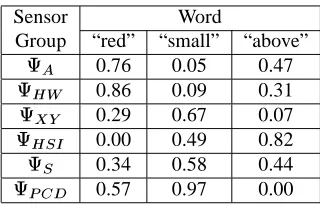
Recurring patterns were discovered in the audio wave-forms corresponding to the utterances (Oates, 2001) and these patterns were used as candidate words. Recall that a sensor group is semantically associated with a word when the mutual information between occurrences of the word and values in the sensor groups are statistically signifi-cant. Table 1 shows the values for the mutual informa-tion for a number of combinainforma-tions of words and sensor groups. Note from the first column that it is clear that the meaning of the word “red” is grounded in the sen-sor group. It is the only one with a statistically significant mutual information value. As the second column indi-cates, the mutual information between the word “small” and the
Table 1: For each sensor group and several words, the cells of the table show the probability of making an error in rejecting the null hypothesis that occurrences of the word and values in the sensor group are independent.
Sensor Word
Group “red” “small” “above”
0.76 0.05 0.47
0.86 0.09 0.31
0.29 0.67 0.07 0.00 0.49 0.82 0.34 0.58 0.44
0.57 0.97 0.00
and the mutual information between this word and the
sensor group is not significant but is rather small. Both of these sensor groups return information about the size of an object, but the
sensor group overesti-mates the area of non-rectangular objects because it re-turns the height and width of a bounding box around an object. Finally, note from the third column that the de-notation of the word “above” is correctly determined to lie in the
sensor group, yet there appears to be some relationship between this word and the
sen-sor group. The reason for this is that objects that are said to be “above” tend to be much higher in the robot’s visual field than all of the other objects.
How is it possible to determine the extent to which a machine has discovered and represented the semantics of a set of words? We are trying to capture semantic distinc-tions made by humans in natural language communica-tion, so it makes sense to ask a human how successful the system has been. This was accomplished as follows. For each word for which a semantic association was discov-ered, each of the training utterances that used the word were identified. For the scene associated with each utter-ance, the CPF underlying the word was used to identify the most probable referent of the word. For example, if the word in question was “red”, then the mean HSI values of all objects in the scene would be computed and the ob-ject for which the underlying CPF defined over HSI space yielded the highest probability would be deemed to be the referent of that word in that scene. A human subject was then asked if it made sense for that word to refer to that object in that scene.
The percentage of content words (i.e. words like “red” and “large” as opposed to “oh” and “there”) for which a semantic association was discovered was
. Given a semantic association, the two ways that it can be in error are as follows: either the wrong sensor group is selected or the conditional probability field defined over that sen-sor group is wrong. Given all of the configurations for
which a particular word was used, the semantic accuracy is the percentage of configurations that the meaning com-ponent of the word selects an aspect of the configuration that a native speaker of the language says is appropriate. The semantic accuracy was
.
6
Discussion
This paper described a method for recovering the deno-tational meaning of a word, i.e.utter-W
, given a set of sensory observations, each labeled according to whether it co-occurred with an utterance contain-ing the word, i.e. hear-W
. It was shown that
hear-W
is a linear function ofutter-W
where the parameters of the transform are determined by the level of shared attention and the background fre-quency of . Given two weak assumptions about the form ofutter-W
, these parameters can be recov-ered and the transform inverted. The use of mutual in-formation and randomization testing to identify the par-ticular sensor group that captures a word’s meaning was described. It is therefore possible to identify the denota-tional meaning of a word by simply observing the con-texts in which it is and is not used, even in the face of imperfect shared attention and homonymy.
References
Paul R. Cohen. 1995. Empirical Methods for Artificial Intelligence. The MIT Press.
Eugene S. Edgington. 1995. Randomization Tests. Mar-cel Dekker.
Tim Oates. 2001. Grounding Knowledge in Sen-sors: Unsupervised Learning for Language and Plan-ning. Ph.D. thesis, The University of Massachusetts, Amherst.
W. V. O. Quine. 1960. Word and object. MIT Press.
Terry Regier. 1996. The Human Semantic Potential. The MIT Press.