—An Experiment Using a Web Search Engine—
Kumiko Tanaka-Ishii
Graduate School of Information Science and Technology, University of Tokyo
Abstract. Previous works have suggested that the uncertainty of tokens coming after a sequence helps determine whether a given position is at a context boundary. This feature of language has been applied to unsupervised text segmentation and term extraction. In this paper, we fundamentally verify this feature. An experiment was performed using a web search engine, in order to clarify the extent to which this assumption holds. The verification was applied to Chinese and Japanese.
1
Introduction
The theme of this paper is the following assumption:
The uncertainty of tokens coming after a sequence helps determine whether a given position is at a context boundary. (A)
Intuitively, the variety of successive tokens at each character inside a word mono-tonically decreases according to the offset length, because the longer the preced-ing character n-gram, the longer the precedpreced-ing context and the more it restricts the appearance of possible next tokens. On the other hand, the uncertainty at the position of a word border becomes greater and the complexity increases, as the position is out of context. This suggests that a word border can be detected by focusing on the differentials of the uncertainty of branching. This assumption is illustrated in Figure 1. In this paper, we measure this uncertainty of successive tokens by utilizing the entropy of branching (which we mathematically define in the next section).
This assumption dates back to the fundamental work done by Harris [6] in 1955, where he says that when the number of different tokens coming after every prefix of a word marks the maximum value, then the location corresponds to the morpheme boundary. Recently, with the increasing availability of corpora, this characteristic of language data has been applied for unsupervised text segmenta-tion into words and morphemes. Kempe [8] reports an experiment to detect word borders in German and English texts by monitoring the entropy of successive characters for 4-grams. Many works in unsupervised segmentation utilise the fact that the branching stays low inside words but increases at a word or mor-pheme border. Some works apply this fact in terms of frequency [10] [2], while others utilise more sophisticated statistical measures: Sun et al. [12] use mutual information; Creutz [4] use MDL to decompose Finnish texts into morphemes.
R. Dale et al. (Eds.): IJCNLP 2005, LNAI 3651, pp. 93–105, 2005. c
This assumption seems to hold not only at the character level but also at the word level. For example, the uncertainty of words coming after the word sequence, “The United States of”, is small (because the word America is very likely to occur), whereas the uncertainty is greater for the sequence “computa-tional linguistics”, suggesting that there is a context boundary just after this term. This observation at the word level has been applied to term extraction by utilising the number of different words coming after a word sequence as an indicator of collocation boundaries [5] [9].
Fig. 1.Intuitive illustration of a variety of successive tokens and a word boundary
As can be seen in these previous works, the above assumption (A) seems to govern language structure both microscopically at the morpheme level and macroscopically at the phrase level. Assumption (A) is interesting not only from an engineering viewpoint but also from a language and cognitive science view-point. For example, some recent studies report that the statistical, innate struc-ture of language plays an important role in children’s language acquisition [11]. Therefore, it is important to understand the innate structure of language, in order to shed light on how people actually acquire it.
Consequently, this paper verifies assumption (A) in a fundamental manner. We address the questions of why and to what extent (A) holds. Unlike recent, previous works based on limited numbers of corpora, we use a web search engine to obtain statistics, in order to avoid the sparseness problem as much as pos-sible. Our discussion focuses on correlating the entropy of branching and word boundaries, because the definition of a word boundary is clearer than that of a morpheme or phrase unit. In terms of detecting word boundaries, our experi-ments were performed in character sequence, so we chose two languages in which segmentation is a crucial problem: Chinese which contains only ideograms, and Japanese, which contains both ideograms and phonograms. Before describing the experiments, we discuss assumption (A) in more detail.
2
The Assumption
Fig. 2.Decrease inH(X|Xn) for characters whennis increased
H(X|Xn) =−
xn∈χn
P(Xn=xn)
x∈χ
P(X =x|Xn=xn) logP(X =x|Xn=xn)
whereP(X=x) indicates the probability of occurrence ofx.
A well-known observation on language data states that H(X|Xn) decreases asnincreases [3]. For example, Figure 2 shows the entropy values asnincreases from 1 to 9 for a character sequence. The two lines correspond to Japanese and English data, from corpora consisting of the Mainichi newspaper (30 MB) and the WSJ (30 MB), respectively. This phenomenon indicates thatX will become easier to estimate as the context of Xn gets longer. This can be intuitively understood: it is easy to guess that “e” will follow after “Hello! How ar”, but it is difficult to guess what comes after the short string “He”.
The last term −log P(X = x|Xn = xn) in formula above indicates the information of a token of xcoming after xn, and thus the branching after xn. The latter half of the formula, the local entropy value for a givenxn
H(X|Xn=xn) =−
x∈χ
P(X =x|Xn=xn) logP(X =x|Xn=xn), (1)
indicates the average information of branching for aspecificn-gram sequencexn.
As our interest in this paper is this local entropy, we denote simplyH(X|Xn= xn) ash(xn) in the rest of this paper.
The decrease inH(X|Xn) globally indicates that given ann-length sequence
xn and another (n+ 1)-length sequenceyn+1, the following inequality holdson
average:
h(xn)> h(yn+1). (2)
One reason why inequality (2) holds for language data is that there iscontextin language, andyn+1 carries a longer contextas compared withxn. Therefore, if
we suppose that xn is the prefix ofxn+1, then it is very likely that
h(xn)> h(xn+1) (3)
holds, because the longer the preceding n-gram, the longer thesamecontext. For example, it is easier to guess what comes after x6=“natura” than what comes
Fig. 3.Our model for boundary detection based on the entropy of branching
concept that if the context is longer, the uncertainty of the branching decreases on average. Then, taking the logical contraposition, if the uncertainty does not decrease, the context is not longer, which can be interpreted as the following:
If the complexity of successive tokens increases, the location is at the context border. (B)
For example, in the case of x7 = “natural”, the entropy h(“natural”) should
be larger thanh(“natura”), because it is uncertain what character will allowx7
to succeed. In the next section, we utilise assumption (B) to detect the context boundary.
3
Boundary Detection Using the Entropy of Branching
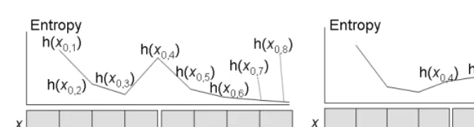
Assumption (B) gives a hint on how to utilise the branching entropy as an indicator of the context boundary. When two semantic units, both longer than 1, are put together, the entropy would appear as in the first figure of Figure 3. The first semantic unit is from offsets 0 to 4, and the second is from 4 to 8, with each unit formed by elements ofχ. In the figure, one possible transition of branching degree is shown, where the plot at k on the horizontal axis denotes the entropy forh(x0,k) andxn,mdenotes the substring between offsetsnandm.
Ideally, the entropy would take a maximum at 4, because it will decrease as
k is increased in the ranges ofk <4 and 4< k <8, and at k= 4, it will rise. Therefore, the position atk= 4 is detected as the “local maximum value” when monitoringh(x0,k) overk. The boundary condition after such observation can
be redefined as the following:
Bmax Boundaries are locations where the entropy is locally maximised.
A similar method is proposed by Harris [6], where morpheme borders can be detected by using the local maximum of the number of different tokens coming after a prefix.
This only holds, however, for semantic units longer than 1. Units often have a length of 1: at the character level, in Japanese and Chinese, there are many one-character words, and at the word level, there are many single words that do not form collocations. If a unit has length 1, then the situation will look like the second graph in Figure 3, where three semantic units,x0,4,x4,5x5,8, are present,
Atk= 5, the value may increase or decrease, because the longer context results in an uncertainty decrease,though an uncertainty decrease does not necessarily mean a longer context. Whenhincreases atk= 5, the situation would look like the second graph. In this case, the condition Bmaxwill not suffice, and we need
a second boundary condition:
Bincrease Boundaries are locations where the entropy is increased.
On the other hand, when hdecreases at k = 5, then even Bincreasecannot be
applied to detectk= 5 as a boundary. We have other chances to detectk= 5, however, by considering h(xi,k) where 0 < i < k. According to inequality (2), then, a similar trend should be present for plots ofh(xi,k), assumingh(x0,n)> h(x0,n+1); then, we have
h(xi,n)> h(xi,n+1), for 0< i < n. (4)
The value h(xi,k) would hopefully rise for some i if the boundary at k = 5 is important, althoughh(xi,k) can increase or decrease atk= 5, just as in the case forh(x0,n).
Therefore, when the target language consists of many one element units, Bincreaseis crucial for collecting all boundaries. Note that boundaries detected
by Bmaxare included in those detected by the condition Bincrease.
Fig. 4.Kempe’s model for boundary detection
Kempe’s detection model is based solely on the assumption that the un-certainty of branching takes a local maximum at a context boundary. Without any grounding on this assumption, Kempe [8] simply calculates the entropy of branching for a fixed length of 4-grams. Therefore, the length of n is set to 3,
h(xi−3,i) is calculated for alli, and the maximum values are claimed to indicate
the word boundary. This model is illustrated in Figure 4, where the plot at each
kindicates the value ofh(xk−3,k). Note that atk= 4, thehvalue will be highest.
It is not possible, however, to judge whetherh(xi−3,i) is larger thanh(xi−2,i+1)
in general: Kempe’s experiments show that thehvalue simply oscillates at a low value in such cases.
Summarising what we have examined, in order to verify assumption (A), which is replaced by assumption (B), the following questions must be answered experimentally:
Q1 Does the condition described by inequality (3) hold? Q2 Does the condition described by inequality (4) hold?
Q3 To what extent are boundaries extracted by Bmaxor Bincrease?
In the rest of this paper, we demonstrate our experimental verification of these questions.
So far, we have considered only regular order processing: the branching degree is calculated forsuccessiveelements ofxn. We can also consider the reverse order,
which involves calculating hfor the previous element of xn. In the case of the
previous element, the question is whether the head ofxn forms thebeginningof
a context boundary. We use the subscriptssuc andprevto indicate the regular and reverse orders, respectively. Thus, the regular order is denoted ashsuc(xn),
while the reverse order is denoted byhprev(xn).
In the next section, we explain how we measure the statistics ofxn, before proceeding to analyze our results.
4
Measuring Statistics by Using the Web
In the experiments described in this paper, the frequency counts were obtained using a search engine. This was done because the web represents the largest pos-sible database, enabling us to avoid the data sparseness problem to the greatest extent possible.
Given a sequencexn,h(xn) is measured by the following procedure. 1. xn is sent to a search engine.
2. One thousand snippets, at maximum, are downloaded and xn is searched for through these snippets. If the number of occurrences is smaller than N, then the system reports thatxn is unmeasurable.
3. The elements occurring before and after xn are counted, andhsuc(xn) and
hprev(xn) are calculated.
N is a parameter in the experiments described in the following section, and a higher N will give higher precision and lower recall. Another aspect of the experiment is that the data sparseness problem quickly becomes significant for longer strings. To address these issues, we choseN=30.
The value of his influenced by the indexing strategy used by a given search engine. Defining f(x) as the frequency count for string x as reported by the search engine,
f(xn)> f(xn+1) (5)
should usually hold ifxnis a prefix ofxn+1, because all occurrences ofxncontain
occurrences of xn+1. In practice, this does not hold for many search engines,
namely, those in whichxn+1is indexed separately fromxn and an occurrence of
xn+1 is not included in one ofxn. For example, the frequency count of “mode”
Fig. 5.Entropy changes for a Japanese character sequence (left:regular; right:reverse)
search engines use this indexing strategy at the string level for languages in which words are separated by spaces, and in our case, we need a search engine in which the count of xn includes that of xn+1. Although we are interested in
the distribution of tokens coming after the string xn and not directly in the
frequency, a larger value off(xn) can lead to a larger branching entropy.
Among the many available search engines, we decided to use AltaVista, be-cause its indexing strategy seems to follow inequality (5) better than do the strategies of other search engines. AltaVista used to utilise string-based index-ing, especially for non-segmented languages. Indexing strategies are currently trade secrets, however, so companies rarely make them available to the pub-lic. We could only guess at AltaVistafs strategy by experimenting with some concrete examples based on inequality (5).
5
Analysis for Small Examples
We will first examine the validity of the previous discussion by analysing some small examples. Here, we utilise Japanese examples, because this language con-tains both phonograms and ideograms, and it can thus demonstrate the features of our method for both cases.
The two graphs in Figure 5 show the actual transition of hfor a Japanese sentence formed of 11 characters:x0,11= (We think of
the future of(natural)language processing(studies)). The vertical axis represents the entropy value, and the horizontal axis indicates the offset of the string. In the left graph, each line starting at an offset ofm+1 indicates the entropy values of hsuc(xm,m+n) for n > 0, with plotted points appearing at k = m+n. For
example, the leftmost solid line starting at offsetk= 1 plots thehvalues ofx0,n
forn >0, withm=0 (refer to the labels on some plots):
x0,1 =
x0,2 =
. . .
x0,5 =
with each value ofhfor the above sequencex0,nappearing at the location ofn.
言語処理の未来を考える
Concerning this line, we may observe that the valueincreasesslightly at po-sitionk= 2, which is the boundary of the word (language). This location will become a boundary for both conditions, Bmaxand Bincrease. Then, at
posi-tionk = 3, the value drastically decreases, because the character coming after (language proce) is limited (as an analogy in English,ssing is the major candidate that comes after language proce). The value rises again atx0,4,
be-cause the sequence leaves the context of (language processing). This location will also become a boundary whether Bmaxor Bincreaseis chosen. The
line stops at n = 5, because the statistics of the strings x0,n for n > 5 were
unmeasurable.
The second leftmost line starting from k = 2 shows the transition of the entropy values of hsuc(x1,1+n) for n > 0; that is, for the strings starting from
the second character , and so forth. We can observe a trend similar to that of the first line, except that the value also increases at 5, suggesting that
k= 5 is the boundary, given the condition Bincrease.
The left graph thus contains 10 lines. Most of the lines are locally maximized or become unmeasurable at the offset ofk= 5, which is the end of a large portion of the sentence. Also, some lines increase at k = 2, 4, 7, and 8, indicating the ends of words, which is correct. Some lines increase at low values at 10: this is due to the verb (think), whose conjugation stem is detected as a border.
Similarly, the right-hand graph shows the results for the reverse order, where each line ending at m−1 indicates the plots of the value of hprev(xm−n,m) for n >0, with the plotted points appearing at positionk=m−n. For example, the rightmost line plotshfor strings ending with (fromm= 11 andn= 10 down to 5):
where x4,11 became unmeasurable. The lines should be analysed from back to
front, where the increase or maximum indicates thebeginningof a word. Overall, the lines ending at 4 or 5 were unmeasurable, and the values rise or take a maximum atk= 2, 4 or 7.
Note that the results obtained from the processing in each direction differ. The forward pass detects 2,4,5,7,8, whereas the backward pass detects 2,4,7. The forward pass tends to detect theendof a context, while the backward pass typically detects the beginning of a context. Also, it must be noted that this analysis not only shows the segmenting position but also the structure of the sentence. For example, a rupture of the lines and a large increase inhare seen atk= 5, indicating the large semantic segmentation position of the sentence. In the right-hand graph, too, we can see two large local maxima at 4 and 7. These segment the sentence into three different semantic parts.
Fig. 6.Other segmentation examples
On these two graphs, questions Q1 through Q3 from§3 can be addressed as follows. First, as for Q1, the condition indicated by inequality (3) holds in most cases where all lines decrease at k= 3,6,9, which correspond to inside words. There is one counter-example, however, caused by conjugation. In Japanese con-jugation, a verb has a prefix as the stem, and the suffix varies. Therefore, with our method, the endpoint of the stem will be regarded as the boundary. As con-jugation is common in languages based on phonograms, we may guess that this phenomenon will decrease the performance of boundary detection.
As for Q2, we can say that the condition indicated by inequality (4) holds, as the upward and downward trends at the same offset k look similar. Here too, there is a counter-example, in the case of a one element word, as indicated in §3. There are two one-word words x4,5= and x7,8= , where the
gradients of the lines differ according to the context length. In the case of one of these words,h can rise or fall between two successive boundaries indicating a beginning and end. Still, we can see that this is complemented by examining lines starting from other offsets. For example, atk= 5, some lines end with an increase.
As for Q3, if we pick boundary condition Bmax, by regarding any
unmeasur-able case ash=−∞, and any maximum of any line as denoting the boundary, then the entry string will be segmented into the following:
This segmentation result is equivalent to that obtained by many other Japanese segmentation tools. Taking Bincreaseas the boundary condition, another
bound-ary is detected in the middle of the last verb (think, segmented at
(
language
)
j(
processing
)
j(
of
)
j(
future
)
j(
of
)
j(
think
).
の を
言語 処理 未来 を 考える
the stem of the verb)”. If we consider detecting the word boundary, then this segmentation is incorrect; therefore, to increase the precision, it would be better to apply a threshold to filter out cases like this. If we consider the morpheme level, however, then this detection is not irrelevant.
These results show that the entropy of branching works as a measure of context boundaries, not only indicating word boundaries, but also showing the sentence structure of multiple layers, at the morpheme, word, and phrase levels. Some other successful segmentation examples in Chinese and Japanese are shown in Figure 6. These cases were segmented by using Bmax. Examples 1
through 4 are from Chinese, and 5 through 12 are from Japanese, where ‘|’ indi-cates the border. As this method requires only a search engine, it can segment texts that are normally difficult to process by using language tools, such as insti-tution names (5, 6), colloquial expressions (7 to 10), and even some expressions taken from Buddhist scripture (11, 12).
6
Performance on a Larger Scale
6.1 Settings
In this section, we show the results of larger-scale segmentation experiments on Chinese and Japanese. The reason for the choice of languages lies in the fact that the process utilised here is based on the key assumption regarding the semantic aspects of language data. As an ideogram already forms a semantic unit as itself, we intended to observe the performance of the procedure with respect to both ideograms and phonograms. As Chinese contains ideograms only, while Japanese contains both ideograms and phonograms, we chose these two languages.
Because we need correct boundaries with which to compare our results, we utilised manually segmented corpora: the People’s Daily corpus from Beijing University [7] for Chinese, and the Kyoto University Corpus [1] for Japanese.
In the previous section, we calculated hfor almost all substrings of a given string. This requires O(n2) searches of strings, with n being the length of the
given string. Additionally, the process requires a heavy access load to the web search engine. As our interest is in verifying assumption (B), we conducted our experiment using the following algorithm for a given stringx.
1. Setm= 0,n=1. 2. Calculatehforxm,n
3. If the entropy is unmeasurable, setm=m+ 1,n=m+ 2, and go to step 2. 4. Compare the result with that forxm,n−1.
5. If the value ofhfulfils the boundary conditions, then outputnas the bound-ary. Setm=m+ 1,n=m+ 2, and go to 2.
6. Otherwise, setn=n+ 1 and go to 2.
The point of the algorithm is to ensure that the string length is not increased once the boundary is found, or if the entropy becomes unmeasurable. This algorithm becomesO(n2) in the worst case where no boundary is found and all substrings
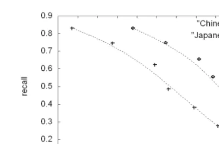
Fig. 7.Precision and recall of word segmentation using the branching entropy in Chi-nese and JapaChi-nese
algorithm defines the regular order case, but we also conducted experiments in reverse order, too.
As for the boundary condition, we utilized Bincrease, as it includes Bmax. A
thresholdvalcould be set to the margin of difference:
h(xn+1)−h(xn)> val. (6)
The largerval is, the higher the precision, and the lower the recall. We varied
valin the experiment in order to obtain the precision and recall curve.
As the process is slow and heavy, the experiment could not be run through millions of words. Therefore, we took out portions of the corpora used for each language, which consisted of around 2000 words (Chinese 2039, Japanese 2254). These corpora were first segmented into phrases at commas, and each phrase was fed into the procedure described above. The suggested boundaries were then compared with the original, correct boundaries.
6.2 Results
The results are shown in Figure 7. The horizontal axis and vertical axes represent the precision and recall, respectively. The figure contains two lines, corresponding to the results for Japanese or Chinese. Each line is plotted by varyingvalfrom 0.0 to 3.0 with a margin of 0.5, where the leftmost points of the lines are the results obtained forval=0.0.
procedure, whereas in the original corpus, complete names are regarded as single words. As another example in Chinese, the character is used to indicate “-ist” in English, as in (revolutionist) and our process suggested that there is a border in between However, in the original corpus, these words are not segmented before but are instead treated as one word. Unlike the precision, the recall ranged significantly according to the thresh-old. Whenval was high, the recall became small, and the texts were segmented into larger phrasal portions. Some successful examples in Japanese for val=3.0 are shown in the following.
The segments show the global structure of the phrases, and thus, this result demonstrates the potential validity of assumption (B). In fact, such sentence segmentation into phrases would be better performed in a word-based manner, rather than a character-based manner, because our character-based experiment mixes the word-level and character-level aspects at the same time. Some previous works on collocation extraction have tried boundary detection using branching [5]. Boundary detection by branching outputs tightly coupled words that can be quite different from traditional grammatical phrases. Verification of such aspects remains as part of our future work.
Overall, in these experiments, we could obtain a glimpse of language structure based on assumption (B) where semantic units of different levels (morpheme, word, phrase) overlaid one another, as if to form a fractal of the context. The entropy of branching is interesting in that it has the potential to detect all boundaries of different layers within the same framework.
7
Conclusion
We conducted a fundamental analysis to verify that the uncertainty of tokens coming after a sequence can serve to determine whether a position is at a con-text boundary. By inferring this feature of language from the well-known fact that the entropy of successive tokens decreases when a longer context is taken, we examined how boundaries could be detected by monitoring the entropy of successive tokens. Then, we conducted two experiments, a small one in Japanese, and a larger-scale experiment in both Chinese and Japanese, to actually segment words by using only the entropy value. Statistical measures were obtained using a web search engine in order to overcome data sparseness.
Through analysis of Japanese examples, we found that the method worked better for sequences of ideograms, rather than for phonograms. Also, we ob-served that semantic layers of different levels (morpheme, word, phrase) could potentially be detected by monitoring the entropy of branching. In our larger-scale experiment, points of increasing entropy correlated well with word borders
and
{
are
jbig
jproblems
jsuchaspower
References
1. Kyoto University Text Corpus Version 3.0, 2003. http://www.kc.t.u-tokyo.ac.jp/nl-resource/corpus.html.
2. R.K. Ando and L. Lee. Mostly-unsupervised statistical segmentation of japanese: Applications to kanji. InANLP-NAACL, 2000.
3. T.C. Bell, J.G. Cleary, and I. H. Witten.Text Compression. Prentice Hall, 1990. 4. M. Creutz and Lagus K. Unsupervised discovery of morphemes. In Workshop of
the ACL Special Interest Group in Computational Phonology, pages 21–30, 2002. 5. T.K. Frantzi and S. Ananiadou. Extracting nested collocations. 16th COLING,
pages 41–46, 1996.
6. S.Z. Harris. From phoneme to morpheme.Language, pages 190–222, 1955. 7. ICL. People daily corpus, beijing university, 1999. Institute of Computational
Linguistics, Beijing University http://162.105.203.93/Introduction/ corpustag-ging.htm.
8. A. Kempe. Experiments in unsupervised entropy-based corpus segmentation. In Workshop of EACL in Computational Natural Language Learning, pages 7–13, 1999.
9. H. Nakagawa and T. Mori. A simple but powerful automatic termextraction method. InComputerm2: 2nd International Workshop on Computational Termi-nology, pages 29–35, 2002.
10. S. Nobesawa, J. Tsutsumi, D.S. Jang, T. Sano, K. Sato, and M Nakanishi. Seg-menting sentences into linky strings using d-bigram statistics. In COLING, pages 586–591, 1998.
11. J.R. Saffran. Words in a sea of sounds: The output of statistical learning.Cognition, 81:149–169, 2001.
12. M. Sun, Dayang S., and B. K. Tsou. Chinese word segmentation without using lexicon and hand-crafted training data. InCOLING-ACL, 1998.