Cofactorization on Graphics Processing Units

(1)

Cofactorization on Graphics Processing Units

Andrea Miele1_{, Joppe W. Bos}2?_{, Thorsten Kleinjung}1_{, and Arjen K. Lenstra}1 1

LACAL, EPFL, Lausanne, Switzerland

2 _{NXP Semiconductors, Leuven, Belgium}

Abstract. We show how the cofactorization step, a compute-intensive part of the relation

collection phase of the number field sieve (NFS), can be farmed out to a graphics processing unit. Our implementation on a GTX 580 GPU, which is integrated with a state-of-the-art NFS implementation, can serve as a cryptanalytic co-processor for several Intel i7-3770K quad-core CPUs simultaneously. This allows those processors to focus on the memory-intensive sieving and results in more useful NFS-relations found in less time.

Keywords:Cofactorization, Graphics Processing Unit, Number Field Sieve

1 Introduction

Today, the asymptotically fastest publicly known integer factorization method is the number field sieve (NFS, [46, 30]). It has been used to set several integer factorization records, most recently a 768-bit RSA modulus as described in [27]. In the first of its two main steps, pairs of integers calledrelations are collected. This is done by iterating a two-stage approach:sieving to collect a large batch of promising pairs, followed by the identification of the relatively few relations among them. Sieving requires a lot of memory and is commonly done on CPUs. The follow-up stage requires little memory and can be parallelized in multiple ways. It may therefore be cost-effective to offload this follow-up stage to a coprocessor. Most previous work in this direction focussed on offloading the elliptic curve integer factoring (ECM, [31]), which is only part of this follow-up stage. For graphics processing units (GPUs) this is considered in [7, 5, 10] and for reconfigurable hardware such as field-programmable gate arrays in [53, 45, 17, 14, 19, 32, 58]. To allow the CPUs to keep sieving, thus optimally using their memory, in this paper the possibility is explored to offload the entire follow-up stage to GPUs. We describe our approach, with a focus on modular and elliptic curve arithmetic, to do so on the many-core, memory-constrained GPU platform. Our results demonstrate that GPUs can be used as an efficienthigh-throughput co-processor for this application.

Our design strategy exploits the inherent task parallelism of the stage that follows the actual sieving, namely the fact that collected pairs can be processed independently in parallel. Because the integers involved are relatively small (at most 384 bits for our target number), we have chosen not to parallelize the integer arithmetic, thereby avoiding performance penalties due to inter-thread synchronization while maximizing the compute-to-memory-access ratio [5]. We use a single thread to process a single pair from the input batch, aiming to maximize the number of pairs processed per second. Because this requires a large number of registers per thread and potentially reduces the GPU utilization, we use integer arithmetic algorithms that minimize register usage and apply native multiply-and-add instructions wherever possible.

For each pair the follow-up stage consists of checking if two integer values, obtained by evaluating two bivariate integer polynomials at the point determined by the pair, are both

?_{Part of this work has been performed while the second author was working for Microsoft Research, WA,}

(2)

smooth, i.e., divisible by primes up to certain bounds. This is done sequentially: a first kernel filters the pairs for which the first polynomial value is smooth, once enough pairs have been collected a second kernel does the same for the second polynomial value, and pairs that pass both filters correspond to relations. Each kernel first computes the relevant polynomial value and then subjects it to a sequence of occasional compositeness tests and factorization attempts aimed at finding small factors.

We have determined good parameters for two different approaches: to find as many rela-tions as possible (≈99% in a batch) and a faster one to find most relations (≈95% in a batch). The effectiveness of these approaches is demonstrated by integrating the GPU software with state-of-the-art NFS software [16] tuned for the factorization of the 768-bit modulus from [27]. A single GTX 580 GPU can serve between 3 and 10 Intel i7-3770Kquad-core CPUs.

Cryptologic applications of GPUs have been considered before: symmetric cryptography in [33, 20, 56, 21, 44, 11, 18], asymmetric cryptography in [39, 54, 22] for RSA and in [54, 1, 9] for ECC, and enhancing symmetric [8] and asymmetric [7, 5, 6, 10] cryptanalysis.

Our source code will be made available.

2 Preliminaries

The Number Field Sieve. For details on how NFS works, see [30, 50]. Its major steps are polynomial selection, relation collection, and the matrix step. For this paper, an operational description of relation collection for numbers in the current range of interest suffices. For those numbers relation collection is responsible for about 90% of the computational effort.

Here we call an integer B-smooth if there is no prime-power larger than B that divides it (elsewhere such numbers are called B-powersmooth). Relation collection uses smoothness bounds Br, Ba ∈Z>0 and polynomialsfr(X), fa(X) ∈Z[X] such that fr is of degree one,fa is irreducible of (small) degreed >1, andfr andfa have a common root modulo the number to be factored. The polynomialsfr and fa are commonly referred to as therational and the algebraic polynomial, respectively. A relation is a pair of coprime integers (a, b) with b > 0 such thatbfr(a/b) isBr-smooth andbdfa(a/b) isBa-smooth.

(3)

follows that ˜t such that t = (x±y) modm is calculated as ˜t = (˜x±y) mod˜ m, and that ˜

s such that s= xy modm satisfies ˜s = ˜x˜yr−kmodm. This Montgomery product ˜s can be computed by first calculating the ordinary integer product u = ˜xy, and by next performing˜ Montgomery reduction: modulo m divide u by rk by replacing k times in succession u by (u+[((umodr)µ) modr]m)/r, then ˜s=u−mifu≥mand ˜s=uotherwise. If 0≤x,˜ y < m,˜ then the same bound hold for ˜s.

Jebelean’s exact division.Ifnis known to be an integer multiple of an odd integerp, the quotient n_p can be computed using an iteration very similar to Montgomery reduction: let µ=−p−1 modr, thenv= ((nmodr)(r−µ)) modr equals the least significant radix-rblock

n

p modr of n

p, after which nis replaced by (n−vp)/rand the other radix-r blocks of n p are

iteratively computed in the same way. This is known asJebelean’s exact division method [24].

3 Cofactoring Steps

This section lists the steps used to identify the relations among a collection of pairs of integers (a, b) that results from NFS sieving for one or more special primes. See [26] for related previous work. The notation is as in Section 2.

For all collected pairs (a, b) the valuesbfr(a/b) andbdfa(a/b) can be calculated by observ-ing thatbkf(a/b) = Pk

i=0fiaibk−i for f(X) =Pik=0fiXi ∈Z[X]. The valuez=bkf(a/b) is

trivially calculated ink(k−1) multiplications by initializingzas 0, and by replacing, fori= 0, 1, . . ., k in succession, z by z+fiaibk−i, or, at the cost of an additional memory location,

in 3k−1 multiplications by initializingz =f0 and t=a and by replacing, fori= 1, 2, . . ., k in succession, z by zb+fitand, if i < k, t by ta. Even with the most naive approach (as

opposed to asymptotically faster methods), this is a negligible part of the overall calculation. The resulting values need to be tested for smoothness, with boundBr for the bfr(a/b)-values and boundBa for thebdfa(a/b)-values.

For all pairs (a, b) bothbfr(a/b) andbdfa(a/b) have relatively many small factors (because the pairs are collected during NFS sieving). After shifting out all factors of two, other very small factors may be found using trial division, somewhat larger ones by Pollardp−1 [47], and the largest ones using ECM [31]. These three methods are further described below. In our experiment (cf. 5.2) it turned out to be best to skip trial division forbfr(a/b) and let Pollard p−1 and ECM take care of the very small factors as well. Based on the findings reported in [28] or their GPU-incompatibility, other integer factorization methods like Pollard rho [48] or quadratic sieve [49] are not considered. It is occasionally useful to make sure that remaining cofactors are composite. An appropriate compositeness test is therefore described first. Compositeness test.Letm−1 = 2tu fort∈Z≥0 and oddu∈Z. If for somea∈(Z/mZ)∗ it is the case that au 6≡ 1 modm and au2i 6≡ −1 modm for 0≤ i < t, then m is composite and a is a witness to m’s compositeness. As shown in [34, 51], for composite m more than 75% of the integers in{1,2, . . . , m−1} are witnesses tom’s compositeness.

(4)

Trial division.Given an odd integern, all its prime factors up to some small trial division bound are removed using trial division. For each small odd prime p (possibly tabulated, if memory is available) firstπ= (−p)−1 modris calculated (per thread, at negligible overhead), withr= 232as in Section 2. Next,nis tested for divisibility byp: withuinitialized asnandk the least integer such thatu < rk, the integeruis modulopdivided byrk(using Montgomery reduction, withp andπ in the roles ofm andµ, respectively). If the resulting 32-bit value u satisfies umodp ≡ 0, then n is divisible by p and the divisibility test is repeated with n replaced by n_p (computed using Jebelean’s method).

Pollard p−1. The prime factors p of n for which p−1 is B1-smooth can be found at a cost ofO(B1) multiplications modulonby means of “stage 1” of Pollard’sp−1 method [47]: with t = ak_mod_{n, for some} _a ₆₌ _±_{1 mod}_n, _a ₆_{= 0 mod}_n _and _k _{the product of all prime}

powers ≤B1, the product of all suchp divides gcd(t−1, n). In practice the value a = 2 is used for efficiency reasons. If the order modulonoftis at mostB2, for some boundB2 > B1, this can be exploited in “stage 2” [36], thereby allowing in p−1 one additional prime factor between B1 and B2. Naively, gcd(t`−1, n) could be computed for all primes ` in (B1, B2]. A much faster but memory-consuming method uses the fast Fourier transform (cf. [38]). On GPUs a baby-step giant-step approach is more suitable and is used here. It follows from the description below and the optimizations described in [36].

Elliptic Curve Method.Stage 1 of Pollard’sp−1 method usesO(B1) multiplications mod-ulonto find prime factorspofnfor which the groups (Z/pZ)∗ haveB1-smooth order. Thus,p can be found in time mostly linear in the largest prime factor ofp−1. The elliptic curve method (ECM) for integer factorization [31] works analogously but replaces the fixed group (Z/pZ)∗ of orderp−1 by a number of groups with orders behaving like random integers close to p: given one such group with B1-smooth order, p can be found in O(B1) multiplications and additions modulon. Trading off the number of groups attempted and the smoothness bound, finding p can heuristically be argued to take exp((√2 +o(1))(√logplog logp)) elementary operations modulon, wherep→ ∞.

Like Pollard’s p−1 method, each ECM attempt operates on a group element and the productkof all prime powers≤B1, mimics the “ mod p” operations by doing them “ mod n”, and hopes to run into the identity element modp but not modn, if not in stage 1 then in stage 2. Where Pollard’s method is based on arithmetic in the group of integers modulo the composite multiple n of p, ECM is based on arithmetic with “points” belonging to groups associated with elliptic curves over prime fields, mimicking those operations by doing them modulo the composite multiple n of those primes. Because the operations may not be well-defined, they may fail, thereby revealing a factor of n.

(5)

order, further enhancing the success probability of ECM (cf. [2, Thm. 3.4 and 3.6] and [3]). More specifically we use “a=−1” twisted Edwards curve (E :−x2+y2 = 1 +dx2y2) overQ withd=−((g−1/g)/2)4 such that d(d+ 1)6= 0 and g∈Q\ {±1,0}.

Related work on stage 1 of ECM for cofactoring on constrained devices can be found in [53, 45, 17, 14, 19, 32, 58, 7, 5, 10]. Unlike these publications, the GPU-implementation presented here includes stage 2 of ECM, as it significantly improves the performance of ECM.

ECM Stage 2 on GPUs. The fastest known methods to implement stage 2 of ECM are FFT-based [12, 36, 37] and rather memory-hungry, which may explain why earlier constrained device ECM-cofactoring work did not consider stage 2. These methods are also incompatible with the memory restrictions of current GPUs. Below a baby-step giant-step approach [52] to stage 2 is described that is suitable for GPUs. Let Q = kP be as above. Similar to the naive approach to stage 2 of Pollard’sp−1 method, the points`Qfor the primes`in (B1, B2] can be computed and be compared to the zero point modulo a prime p dividing n but not modulon by computing the gcd of nand the product of the x-coordinates of the points `Q. WithN primes`, computing all points requires about 8N multiplications inZ/nZ, assuming a few precomputed small even multiples ofQ. Balancing the computational efforts of the two stages withB1= 256 as above, leads toB2 = 2803 (andN = 354).

The baby-step giant step approach from [36] speeds up the calculation at the cost of more memory, while also exploiting that for Edwards curves and any point P it is the case that

y(P) t(P) =

y(−P)

t(−P), (1)

withy(P) andt(P) they- and t-coordinate, respectively, of P.

For a giant-step value w < B1, any ` as above can be written as vw ±u where u ∈

U =u∈Z : 1≤u≤ w

2,gcd(u, w) = 1 , andv∈V =

v∈Z : B1

w −

1 2

≤v≤_B₂ w +

1 2 . Comparing (vw − u)Q to the zero point modulo p but not modulo n amounts to checking if gcd(t(uQ)y(vwQ) − t(vwQ)y(uQ), n) 6= 1. Because of (1), this compares (vw + u)Q to the zero point as well. Hence, computation of gcd(m, n) for m =

Q v∈V

Q

u∈U(t(uQ)y(vwQ)−t(vwQ)y(uQ)) suffices to check ifQhas prime order in (B1, B2]. Optimal parameters balance the costs of the preparation of the ϕ(₂w) tabulated baby-step val-ues (y(uQ) : t(uQ)) (where ϕ is Euler’s totient function) and on the fly computation of the giant-step values (y(vwQ) : t(vwQ)). Suboptimal, smaller w-values may be used to reduce storage requirements. For instance, the choice w = 2·3·5·7 and B2 = 7770 leads to 24 tabulated values and a total of 2904 multiplications and squarings modulo n, which matches the computational effort of stage 1 with B1 = 256. Although gcd(u, w) = 1 already avoids easy composites, the product can be restricted to those u, v for which one ofvw±u is prime if storage for about B2−B1

w ×

ϕ(w)

2 bits is available. With w and tabulated baby-step values as above, this increasesB2 to 8925 for a similar computational effort, but requires about 125 bytes of storage. A more substantial improvement is to define

yv=

Y

˜

v∈V−{v}

t(˜vwQ) Y ˜

u∈U

t(˜uQ)y(vwQ) andyu =

Y

˜

u∈U−{u}

t(˜uQ) Y ˜

v∈V

t(˜vwQ)y(uQ),

and to replacem by Q v∈V

Q

u∈U(yv−yu). This saves 2|V||U|of the 3|V||U|multiplications

in the calculation ofm at a cost that is linear in |U|+|V|to tabulate theyv and yu values.

(6)

4 GPU Implementation Details

In this section we outline our approach to implement the algorithms from Section 3 with a focus on the many-core GPU architecture. We used a quad-core Intel i7-3770K CPU running at 3.5 GHz with 16 GB of memory and an NVIDIA GeForce GTX 580 GPU, with 512 CUDA cores running at 1544 MHz and 1.5 GB of global memory, as further described below.

4.1 Compute unified device architecture

We focus on the GeForce x-series families for x ∈ {8,9,100,200,400,500,600,700}, of the NVIDIA GPU architecture with the compute unified device architecture (CUDA) [41]. Our NVIDIA GeForce GTX 580 GPU belongs to the GeForce 400- and 500-series ([40]) of the Fermi architecture family. These GPUs support 32×32→32-bit multiplication instructions, for both the least and most significant 32 bits of the result.

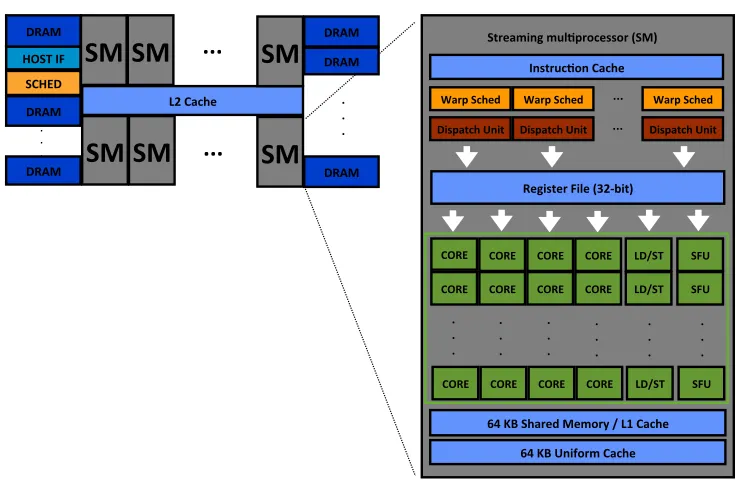
Each GPU contains a number of streaming multiprocessors (SMs), with each SM consisting of multiple scalar processor cores (SP). On a Fermi architecture GPU there are typically about 16 SMs and 32 SPs per SM, but numbers vary per model. Figure 1 depicts a high-level overview of a CUDA GPU architecture.

CORE CORE CORE CORE

64 KB Shared Memory / L1 Cache Register File (32-‐bit)

64 KB Uniform Cache InstrucIon Cache

Warp Sched

Dispatch Unit

. . .

Streaming mulIprocessor (SM)

L2 Cache

...

HOST IF SCHED DRAM

SM

SM SM

SM

...

LD/ST

LD/ST SFU

SFU LD/ST SFU Warp Sched

Dispatch Unit Warp Sched

Dispatch Unit

. . .

. . . ...

... DRAM

DRAM

DRAM . . .

. . .

DRAM DRAM

(7)

C for CUDA is an extension to the C language that employs thesingle-instruction multiple-thread (SIMT) model of massively parallel programming. The programmer defines kernel functions, which are compiled for and executed in parallel on the SPs such that each light-weight thread executes the same instructions but on its own data. A number of threads is grouped into athread blockwhich is scheduled on a single SM, the threads of which time-share the SPs.

Threads inside a thread block are executed in groups of 32 called warps. On Fermi ar-chitecture GPUs each SM has two warp schedulers and two instruction dispatch units. This means that two instructions, from separate warps, can be scheduled and dispatched at the same time. Switching between warps, filling the pipeline as much as possible, a high through-put rate can be sustained. The distinct possibilities of a conditional branch are executed serially by the threads inside a warp, with threads active only when their branch is executed. Multiple execution paths within a warp are thus best avoided.

Threads in the same block can communicate via on-chip shared memory and may syn-chronize their execution using barriers (a synchronization method which makes threads wait until all reach a certain point). There is a large but relatively slow amount of global memory that is accessible to all threads. Fermi architecture GPUs have an L1-cache for each SM, and a unified L2-cache together with fast constant (read-only) memory initialized by the CPU.

4.2 Modular arithmetic on GPUs

We used the parallel thread execution (PTX) instruction set and inline assembly wherever possible to simplify (cf. carry-handling) and speed-up (cf. multiply-and-add) our code; Table 7 in the Appendix lists the arithmetic assembly routines used. “Warp divergent” code was reduced to a minimum by converting most branches intostraight line code to avoid different execution paths within a warp: branch-free code that executes both branches and uses a bit-mask to select the correct value was often found to be more efficient than “if-else” statements. Practical performance.Our decision not to use parallel integer arithmetic dictates the use of algorithms with minimal register usage. For Montgomery multiplication, the most critical operation, we therefore preferred the plain interleaved schoolbook method to Karatsuba [25]; Algorithm 6 in the Appendix gives the CUDA pseudo-code for moduli of at least 96 bits.

Table 1 compares our results both with the state-of-the-art implementation from [29] benchmarked on an NVIDIA GTX 480 card (480 cores, 1401Mhz) and with the ideal peak throughput attainable on our GTX 580 GPU. Compared to [29] our throughput is up to twice better, especially for smaller (128-bit) moduli, even after the figures from [29] are scaled by a factor of 512₄₈₀ · 1544

(8)

Table 1.Benchmark results for the NVIDIA GTX 580 GPU for number of Montgomery multiplications per second and ECM trials per second for various modulus sizes. The Montgomery multiplication throughput reported in [29] was scaled as explained in the text. The estimated peak throughput based on an instruction count is also included together with the total number of dispatched threads. ECM used boundsB1= 256 and B2= 16384 (for a total of 2844 + 3368 = 6212 Montgomery multiplications per trial).

Leboeuf [29] this work

Montgomery multiplications ECM (8192 threads for all sizes) moduli measured measured peak #threads trials Montgomery multiplications

bitsize (scaled, millions) (millions) (thousands) measured (millions)

96 10119 10135 16384 1078 6697

128 2799 5805 5813 16384 674 4187

160 2261 3760 3764 16384 453 2814

192 1837 2631 2635 16384 309 1920

224 1507 1943 1947 15360 243 1510

256 1212 1493 1497 10240 180 1118

320 828 962 964 10240 107 665

384 600 671 672 9216 86 534

as one of the next inputs) before transferring the results back to the CPU. Our throughput turns out to be very close to the peak value.

4.3 Elliptic curve arithmetic on GPUs

When running stage 1 of ECM on memory constrained devices like GPUs, the large number of precomputed points required for windowing methods cannot be stored in fast memory. Thus, one is forced to settle for a (much) smaller window size, thereby reducing the advantage of using twisted Edwards curves. For example, in [7] windowing is not used at all because, citing [7], “Besides the base point, we cannot cache any other points”. Memory is also a problem in [5], where the faster curve arithmetic from Hisil et al. [23] is not used since this requires storing a fourth coordinate per point. These concerns were the motivation behind [10], the approach we adopted for stage 1 of ECM (as indicated in Section 3). For stage 2 we use the baby-step giant-step approach, optimized as described at the end of Section 3 forB2≤32768. Using bounds that balance the number of stage 1 and 2 multiplications does not necessarily balance the GPU running time of the two stages (this varies with the modulus size), but it is a good starting point for further optimization.

(9)

5 Cofactorization on GPUs

This section describes our GPU approach to cofactoring, i.e., recognizing among the pairs (a, b) resulting from NFS sieving those pairs for whichbfr(a/b) isBr-smooth andbdfa(a/b) is Ba-smooth. Approaches common on regular cores (resieving followed by sequential processing of the remaining candidates) allow pair-by-pair optimization with respect to the highest overall yield or yield per second while exploiting the available memory, but are incompatible with the memory and SIMT restrictions of current GPUs.

5.1 Cofactorization overview

Given our application, where throughput is important but latency almost irrelevant, it is a natural choice to process each pair in a single thread, eliminating the need for inter-thread communication, minimizing synchronization overhead, and allowing the scheduler to maximize pipelining by interleaving instructions from different warps. On the negative side, the large memory footprint per thread reduces the number of simultaneously active threads per SM.

The cofactorization stage is split into two GPU kernel functions that receive pairs (a, b) as input: the rational kernel outputs pairs for whichbfr(a/b) is Br-smooth to the algebraic kernel that outputs those pairs for which bd_f

a(a/b) is Ba-smooth as well. The two kernels have the same code structure: all that distinguishes them is that the algebraic one usually has to handle larger values and a higher degree polynomial. To make our implementation flexible with respect to the polynomial selection, the maximum size of the polynomial values is a kernel parameter that is fixed at compile time and that can easily be changed together with the polynomial degree and coefficient size and the size of the inputs.

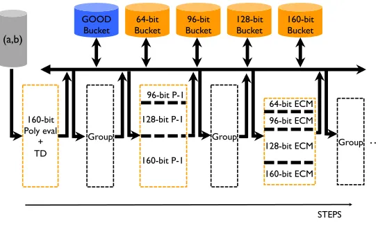
Kernel structure.Given a pair (a, b), a kernel-thread first evaluates the relevant polynomial, storing the odd part n of the resulting value along with identifying information i as a pair (i, n); if applicable the special prime is removed fromn. The value nis then updated in the following sequence of steps, with all parameters set at run-time using a configuration file. First trial division may be applied up to a small bound. The resulting pairs (i, n) are regrouped depending on their radix-232sizes. The cost of the resulting inter-thread communication and synchronization is outweighed by the advantage of being able to run size-specific versions of the other steps. All threads in a warp then grab a pair (i, n) of the same size and each thread attempts to factor its n-value using Pollard’s p−1 method or ECM. If the resulting n is at most the smoothness bound, the kernel outputs the ith pair (a, b). If n’s compositeness cannot be established or ifnis larger than some user-defined threshold, theith pair (a, b) is discarded. Pairs (i, n) with small enough compositenare regrouped and reprocessed. Figure 2 shows a pictorial example of a kernel execution flow.

This approach treats every pair (i, n) in the same group in the same way, which makes it attractive for GPUs. However, unnecessary computations may be performed: for instance, if a factoring attempt fails, compositeness does not need to be reascertained. Avoiding this requires divergent code which, as it turned out, degrades the performance. Also, factoring attempts may chance upon a factor larger than the smoothness bound, an event that goes by unnoticed as only the unfactored part is reported back. We have verified that the CPU easily discards such mishaps at negligible overhead.

(10)

160-bit Poly eval

+

TD

64-bit

Bucket Bucket96-bit 128-bitBucket 160-bitBucket GOOD

Bucket

(a,b)

96-bit P-1

Group

96-bit ECM 64-bit ECM

128-bit ECM

160-bit ECM 128-bit P-1

160-bit P-1

Group

STEPS Group

1

…

Fig. 2.An example of kernel execution flow where the values are assumed to be at most 160 bits. The height

of the dashed rectangles is proportional to the number of values that are processed at a given step.

Table 2.Time in seconds to process a single special prime on all cores of a quad-core Intel i7-3770K CPU.

large number of pairs relations sieving cofactoring total % of time spent relations primes after sieving found time time time on cofactoring per second

3 ≈5·105 ₁₂₅ ₂₅_.₆ ₄_.₀ ₂₉_.₆ ₁₃_.₅ ₄_.₂₂

4 ≈106 137 25.9 6.1 32.0 19.1 4.28

controls the GPU by iterating the following steps (where the roles of the kernels may be reversed and the batch sizes depend on the GPU memory constraints and the kernel):

1. copy a batch from the FIFO buffer to the GPU; 2. launch the rational kernel on the GPU;

3. store the pairs output by the rational kernel in an intermediate buffer; 4. if the intermediate buffer does not contain enough pairs, return to Step 1; 5. copy a batch from the intermediate buffer to the GPU;

6. launch the algebraic kernel on the GPU (providing it with the proper special primes); 7. store the pairs output by the algebraic kernel in a file and return to Step 1.

Exploiting the GPU memory hierarchy.GPU performance strongly depends on where intermediate values are stored. We use constant memory for fixed data precomputed by the CPU and accessed by all threads at the same time: primes for trial division, polynomial coefficients, and baby-step giant-step table-indices for the second stages of factoring attempts. To lower register pressure, the fast shared memory per SM acts as a “user-defined cache” for the values most frequently accessed, such as the moduli n to be factored and the values

(11)

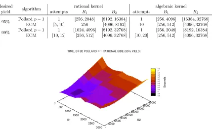
Table 3.Parameters choices for cofactoring. Later ECM attempts use larger bounds in the specified ranges.

desired

algorithm rational kernel algebraic kernel

yield attempts B1 B2 attempts B1 B2

95% Pollardp−1 1 [256,2048] [8192,16384] 1 [256,4096] [16384,32768] ECM [5,10] 256 [4096,8192] 10 [256,512] [4096,32768]

99% Pollardp−1 1 [1024,4096] [8192,32768] 1 [256,2048] [8192,16384] ECM [10,12] [256,512] [4096,32768] [10,20] [256,512] [4096,32768]

0 500

1000 1500

2000 2500

3000 0 5000

10000 15000

20000 25000

30000 35000

40000 TIME, B1 B2 POLLARD P-1 RATIONAL SIDE (95% YIELD)

B1 B2

5.8 5.9 6 6.1 6.2 6.3 6.4 6.5 6.6 6.7 6.8 6.9 7 7.1

Seconds

Fig. 3.Rational kernel cofactoring run times as a function of the Pollardp−1 bounds with desired yield 95%.

5.2 Parameter selection

For our experiments we applied the CPU NFS siever from [16] (obviously, with multi-threading enabled) to produce relations for the 768-bit number from [27]. Except for the special prime, three so-calledlarge primes (i.e., primes not used for sieving but bounded by the applicable smoothness bound) are allowed in the rational polynomial value, whereas on the algebraic side the number of large primes is limited to three or four. Table 2 lists typical figures obtained when processing a single special prime in either setting; the percentages are indicative for NFS factorizations in general. The relatively small amount of time spent by the CPU on cofactoring suggests various ways to select optimal GPU parameters. One approach is aiming for as many relations per second as possible. Another approach is to aim for a certain fixed percentage of the relations among the pairs produced by NFS sieving, and then to select parameters that minimize the GPU time (thus maximizing the number of CPUs that can be served by a GPU). Although in general a fixed percentage cannot be ascertained, it can be done for experimental runs covering a fixed set of special prime ranges, and the resulting parameters can be used for production runs covering all special primes. Here we report on this latter approach in two settings: aiming for all (denoted by “99%”) or for 95% of all relations.

(12)

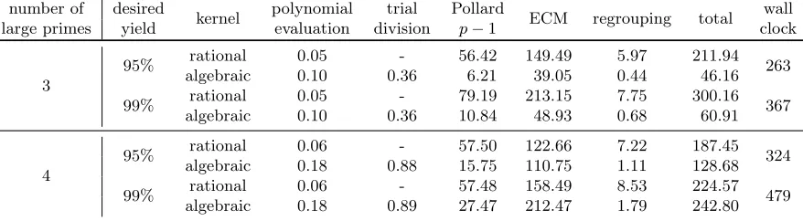
Table 4.Approximate timings in seconds of cofactoring steps to process approximately 50 million (a, b) pairs, measured using the CUDAclock64 instruction. The wall clock time (measured with the unix time utility) includes the kernel launch overhead the CPU/GPU memory transfer and all CPU book-keeping operations.

number of desired

kernel polynomial trial Pollard ECM regrouping total wall large primes yield evaluation division p−1 clock

3

95% rational 0.05 - 56.42 149.49 5.97 211.94 263 algebraic 0.10 0.36 6.21 39.05 0.44 46.16

4

This led to the observations below. Although other input numbers (than our 768-bit modulus) may lead to other choices our results are indicative for generic large composites.

We found that the rational kernel should be executed first, that it is best to skip trial division in the rational kernel, and that a small trial division bound (say, 200) in the algebraic kernel leads to a slight speed-up compared to not using algebraic trial division. For all other steps the two kernels behave similarly, though with somewhat different parameters that also depend on the desired yield (but not on the large prime setting). The details are listed in Table 3. Not shown there are the discarding thresholds that slightly decrease with the number of ECM attempts. Actual run times of the cofactoring steps are given in Table 4. Rational batches contain 3.5 times more pairs than algebraic ones (because the algebraic kernel has to handle larger values). For 3 large primes the rational kernel is called 5 times more often than the algebraic one, for 4 large primes 2.2 times more often.

Varying the bounds of the Pollard p−1 factoring attempt on the rational side within reasonable ranges does not noticeably affect the yield because almost all missed prime factors are found by the subsequent ECM attempts. However, early removal of small primes may reduce the sizes, thus reducing the ECM run time and, if not too much time is spent on Pollard p−1, also the overall run time. This is depicted in Figure 3. Note that in record breaking ECM work the number of trials is much larger; however, according to [55] the empirically determined numbers reported in Table 3 are in the theoretically optimal range.

5.3 Performance results

Table 5 summarizes the results when the same special prime as in Table 2 is processed, but now with GPU-assistance. The figures clearly show that farming out cofactoring to a GPU is

Table 5.GPU cofactoring for a single special prime. The number of quad-core CPUs that can be served by a

single GPU is given in the second to last column.

large number of pairs desired

seconds CPU/GPU relations primes after sieving yield ratio found

3 ≈5·105 95% 2.6 9.8 132 99% 3.7 6.9 136

4 ≈106 95% 6.5 4.0 159

(13)

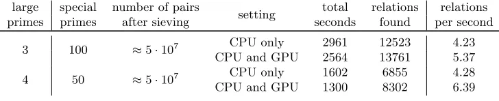
Table 6.Processing multiple special primes with desired yield 99%.

large special number of pairs

setting total relations relations primes primes after sieving seconds found per second

3 100 ≈5·107 CPU only 2961 12523 4.23

CPU and GPU 2564 13761 5.37

4 50 ≈5·107 CPU only 1602 6855 4.28 CPU and GPU 1300 8302 6.39

advantageous from an overall run time point of view and that, depending on the yield desired, a single GPU can keep up with multiple quad-core CPUs. Remarkably, more relations may be found given the same collection of (a, b) pairs: with an adequate number of GPUs each special prime can be processed faster and produces more relations. Based on more extensive experiments the overall performance gain measured in “relations per second” found with and without GPU assistance is 27% in the 3 large primes case and 50% in the 4 large primes case (cf. Table 6).

Including equipment and power expenses in the analysis is much harder, as illustrated by (unrelated) experiments in [43]. Relative power and purchase costs vary constantly, and the power consumption of a GPU running CUDA applications depends on the configuration and the operations performed [13]. For instance, global memory accesses account for a large fraction of the power consumption and the effect on the power consumption of arithmetic instructions depends more on their throughput than on their type. We have not carried out actual power consumption measurements comparing the settings from Table 6.

6 Conclusion

It was shown that modern GPUs can be used to accelerate a compute-intensive part of the relation collection step of the number field sieve integer factorization method. Strategies were outlined to perform the entire cofactorization stage on a GPU. Integration with state-of-the-art lattice siever software indicates that a performance gain of up to 50% can be expected for the relation collection step of factorization of numbers in the current range of interest, if a single GPU can assist a regular multi-core CPU. Because relation collection for such numbers is responsible for about 90% of the total factoring effort the overall gain may be close to 45%; we have no experience with other sizes yet.

It is a subject of further research if a speed-up can be obtained using other types of graphic cards (to which we did not have access). In particular it would be interesting to explore if and how lower-end CUDA enabled GPUs can still be used for the present application and if the larger memory of more recent cards such as the GeForce GTX 780 Ti or GeForce GTX Titan can be exploited. Given our results we consider it unlikely that it would be advantageous to combine multiple GPUs using NVIDIA’s scalable link interface.

Acknowledgements. This work was supported by the Swiss National Science Foundation under grant number 200020-132160. We gratefully acknowledge comments by the anonymous referees.

References

(14)

199, 2010.

2. R. Barbulescu, J. W. Bos, C. Bouvier, T. Kleinjung, and P. L. Montgomery. Finding ECM-friendly curves through a study of Galois properties. In E. W. Howe and K. S. Kedlaya, editors, Algorithmic Number Theory Symposium – ANTS 2012, volume 1 ofThe Open Book Series, pages 63–86. Mathematical Sciences Publishers, 2013.

3. D. J. Bernstein, P. Birkner, and T. Lange. Starfish on strike. In M. Abdalla and P. S. L. M. Barreto, editors,Latincrypt, volume 6212 ofLecture Notes in Computer Science, pages 61–80. Springer, Heidelberg, 2010.

4. D. J. Bernstein, P. Birkner, T. Lange, and C. Peters. ECM using Edwards curves. Mathematics of Computation, 82(282):1139–1179, 2013.

5. D. J. Bernstein, H.-C. Chen, M.-S. Chen, C.-M. Cheng, C.-H. Hsiao, T. Lange, Z.-C. Lin, and B.-Y. Yang. The billion-mulmod-per-second PC. In Special-purpose Hardware for Attacking Cryptographic Systems – SHARCS 2009, pages 131–144, 2009.

6. D. J. Bernstein, H.-C. Chen, C.-M. Cheng, T. Lange, R. Niederhagen, P. Schwabe, and B.-Y. Yang. ECC2K-130 on NVIDIA GPUs. In G. Gong and K. C. Gupta, editors, Progress in Cryptology – IN-DOCRYPT 2010, volume 6498 of Lecture Notes in Computer Science, pages 328–346. Springer-Verlag Berlin Heidelberg, 2010.

7. D. J. Bernstein, T.-R. Chen, C.-M. Cheng, T. Lange, and B.-Y. Yang. ECM on graphics cards. In A. Joux, editor, Eurocrypt 2009, volume 5479 of Lecture Notes in Computer Science, pages 483–501. Springer, Heidelberg, 2009.

8. M. Bevand. MD5 Chosen-Prefix Collisions on GPUs. Black Hat, 2009. Whitepaper.

9. J. W. Bos. Low-latency elliptic curve scalar multiplication.International Journal of Parallel Programming, 40(5):532–550, 2012.

10. J. W. Bos and T. Kleinjung. ECM at work. In X. Wang and K. Sako, editors,Asiacrypt 2012, volume 7658 ofLecture Notes in Computer Science, pages 467–484. Springer Berlin Heidelberg, 2012.

11. J. W. Bos and D. Stefan. Performance analysis of the SHA-3 candidates on exotic multi-core architectures. In S. Mangard and F.-X. Standaert, editors,Cryptographic Hardware and Embedded Systems – CHES 2010, volume 6225 ofLecture Notes in Computer Science, pages 279–293. Springer, Heidelberg, 2010.

12. R. P. Brent. Some integer factorization algorithms using elliptic curves. Australian Computer Science Communications, 8:149–163, 1986.

13. S. Collange, D. Defour, and A. Tisserand. Power consumption of GPUs from a software perspective. In Proceedings of the 9th International Conference on Computational Science: Part I, ICCS ’09, pages 914–923, Berlin, Heidelberg, 2009. Springer-Verlag.

14. G. de Meulenaer, F. Gosset, G. M. de Dormale, and J.-J. Quisquater. Integer factorization based on elliptic curve method: Towards better exploitation of reconfigurable hardware. In Field-Programmable Custom Computing Machines – FCCM 2007, pages 197–206. IEEE Computer Society, 2007.

15. H. M. Edwards. A normal form for elliptic curves.Bulletin of the American Mathematical Society, 44:393– 422, July 2007.

16. J. Franke and T. Kleinjung. GNFS for linux. Software, 2012.

17. K. Gaj, S. Kwon, P. Baier, P. Kohlbrenner, H. Le, M. Khaleeluddin, and R. Bachimanchi. Implementing the elliptic curve method of factoring in reconfigurable hardware. In L. Goubin and M. Matsui, editors, Cryptographic Hardware and Embedded Systems – CHES 2006, volume 4249 ofLecture Notes in Computer Science, pages 119–133. Springer, Heidelberg, 2006.

18. J. Gilger, J. Barnickel, and U. Meyer. GPU-acceleration of block ciphers in the OpenSSL cryptographic library. In D. Gollmann and F. Freiling, editors,Information Security, volume 7483 of Lecture Notes in Computer Science, pages 338–353. Springer Berlin Heidelberg, 2012.

19. T. G¨uneysu, T. Kasper, M. Novotny, C. Paar, and A. Rupp. Cryptanalysis with COPACOBANA. IEEE Transactions on Computers, 57:1498–1513, 2008.

20. O. Harrison and J. Waldron. AES encryption implementation and analysis on commodity graphics pro-cessing units. In P. Paillier and I. Verbauwhede, editors,Cryptographic Hardware and Embedded Systems – CHES 2007, volume 4727 ofLecture Notes in Computer Science, pages 209–226. Springer, Heidelberg, 2007.

21. O. Harrison and J. Waldron. Practical symmetric key cryptography on modern graphics hardware. In Proceedings of the 17th conference on Security symposium, pages 195–209. USENIX Association, 2008. 22. O. Harrison and J. Waldron. Efficient acceleration of asymmetric cryptography on graphics hardware. In

(15)

23. H. Hisil, K. K.-H. Wong, G. Carter, and E. Dawson. Twisted Edwards curves revisited. In J. Pieprzyk, editor, Asiacrypt 2008, volume 5350 of Lecture Notes in Computer Science, pages 326–343. Springer, Heidelberg, 2008.

24. T. Jebelean. An algorithm for exact division. Journal of Symbolic Computation, 15(2):169–180, 1993. 25. A. A. Karatsuba and Y. Ofman. Multiplication of many-digital numbers by automatic computers. Number

145 in Proceedings of the USSR Academy of Science, pages 293–294, 1962.

26. T. Kleinjung. Cofactorisation strategies for the number field sieve and an estimate for the sieving step for factoring 1024-bit integers. InSpecial-purpose Hardware for Attacking Cryptographic Systems – SHARCS 2006, 2006.

27. T. Kleinjung, K. Aoki, J. Franke, A. K. Lenstra, E. Thom´e, J. W. Bos, P. Gaudry, A. Kruppa, P. L. Montgomery, D. A. Osvik, H. te Riele, A. Timofeev, and P. Zimmermann. Factorization of a 768-bit RSA modulus. In T. Rabin, editor, Crypto 2010, volume 6223 of Lecture Notes in Computer Science, pages 333–350. Springer, Heidelberg, 2010.

28. A. Kruppa. A software implementation of ECM for NFS. Research Report RR-7041, INRIA, 2009. http://hal.inria.fr/inria-00419094/PDF/RR-7041.pdf.

29. K. Leboeuf, R. Muscedere, and M. Ahmadi. A GPU implementation of the Montgomery multiplication algorithm for elliptic curve cryptography. In IEEE International Symposium on Circuits and Systems (ISCAS), pages 2593–2596, 2013.

30. A. K. Lenstra and H. W. Lenstra, Jr. The Development of the Number Field Sieve, volume 1554 ofLecture Notes in Mathematics. Springer-Verslag, 1993.

31. H. W. Lenstra, Jr. Factoring integers with elliptic curves. Annals of Mathematics, 126(3):649–673, 1987. 32. D. Loebenberger and J. Putzka. Optimization strategies for hardware-based cofactorization. In M. J. Jacobson Jr., V. Rijmen, and R. Safavi-Naini, editors, Selected Areas in Cryptography – SAC, volume 5867 ofLecture Notes in Computer Science, pages 170–181. Springer, Heidelberg, 2009.

33. S. Manavski. CUDA compatible GPU as an efficient hardware accelerator for AES cryptography. In Signal Processing and Communications, 2007. ICSPC 2007. IEEE International Conference on, pages 65–68, 2007.

34. G. L. Miller. Riemann’s hypothesis and tests for primality. In Proceedings of seventh annual ACM symposium on Theory of computing, STOC ’75, pages 234–239. ACM, 1975.

35. P. L. Montgomery. Modular multiplication without trial division. Mathematics of Computation, 44(170):519–521, April 1985.

36. P. L. Montgomery. Speeding the Pollard and elliptic curve methods of factorization. Mathematics of Computation, 48(177):243–264, 1987.

37. P. L. Montgomery.An FFT extension of the elliptic curve method of factorization. PhD thesis, University of California, 1992.

38. P. L. Montgomery and R. D. Silverman. An FFT extension to the p-1 factoring algorithm. Mathematics of Computation, 54(190):839–854, 1990.

39. A. Moss, D. Page, and N. P. Smart. Toward acceleration of RSA using 3D graphics hardware. In S. D. Galbraith, editor,Proceedings of the 11th IMA international conference on Cryptography and coding, Cryp-tography and Coding 2007, pages 364–383. Springer-Verlag, 2007.

40. NVIDIA. Fermi architecture whitepaper. http://www.nvidia.com/content/PDF/fermi_white_papers/ NVIDIA_Fermi_Compute_Architecture_Whitepaper.pdf, 2010.

41. NVIDIA. Cuda programming guide 5. http://docs.nvidia.com/cuda/cuda-c-programming-guide/ index.html, 2013.

42. NVIDIA. Parallel thread execution isa version 3.2. http://docs.nvidia.com/cuda/parallel-thread-execution/index.html, 2013.

43. NVIDIA Developer Zone. https://devtalk.nvidia.com/default/topic/491799/gtx-590-cuda-power-tests/. 2011.

44. D. A. Osvik, J. W. Bos, D. Stefan, and D. Canright. Fast software AES encryption. In S. Hong and T. Iwata, editors, Fast Software Encryption – FSE 2010, volume 6147 of Lecture Notes in Computer Science, pages 75–93. Springer, Heidelberg, 2010.

45. J. Pelzl, M. ˇSimka, T. Kleinjung, J. Franke, C. Priplata, C. Stahlke, M. Drutarovsk´y, V. Fischer, and C. Paar. Area-time efficient hardware architecture for factoring integers with the elliptic curve method. Information Security, IEE Proceedings on, 152(1):67–78, 2005.

46. J. M. Pollard. The lattice sieve. pages 43–49 in [30].

47. J. M. Pollard. Theorems on factorization and primality testing.Proceedings of the Cambridge Philosophical Society, 76:521–528, 1974.

(16)

49. C. Pomerance. The quadratic sieve factoring algorithm. In T. Beth, N. Cot, and I. Ingemarsson, editors, Eurocrypt 1984, volume 209 of Lecture Notes in Computer Science, pages 169–182. Springer, Heidelberg, 1985.

50. C. Pomerance. A tale of two sieves.Biscuits of Number Theory, 85, 2008.

51. M. O. Rabin. Probabilistic algorithm for testing primality. Journal of Number Theory, 12(1):128–138, 1980.

52. D. Shanks. Class number, a theory of factorization, and genera. In D. J. Lewis, editor,Symposia in Pure Mathematics, volume 20, pages 415–440. American Mathematical Society, 1971.

53. M. ˇSimka, J. Pelzl, T. Kleinjung, J. Franke, C. Priplata, C. Stahlke, M. Drutarovsk´y, and V. Fischer. Hard-ware factorization based on elliptic curve method. InField-Programmable Custom Computing Machines – FCCM 2005, pages 107–116. IEEE Computer Society, 2005.

54. R. Szerwinski and T. G¨uneysu. Exploiting the power of GPUs for asymmetric cryptography. In E. Oswald and P. Rohatgi, editors, Cryptographic Hardware and Embedded Systems – CHES 2008, volume 5154 of Lecture Notes in Computer Science, pages 79–99. Springer, Heidelberg, 2008.

55. G. Xin. Fast smoothness test. Semester project report, June 2013.

56. J. Yang and J. Goodman. Symmetric key cryptography on modern graphics hardware. In K. Kurosawa, editor,Asiacrypt, volume 4833 ofLecture Notes in Computer Science, pages 249–264. Springer, Heidelberg, 2007.

57. P. Zimmermann and B. Dodson. 20 years of ECM. In F. Hess, S. Pauli, and M. E. Pohst, editors, Algorithmic Number Theory – ANTS-VII, volume 4076 ofLecture Notes in Computer Science, pages 525– 542. Springer, Heidelberg, 2006.

(17)

Appendix

Letr= 232.

Table 7.Pseudo-code notation for CUDA PTX assembly instructions [42] used in our implementation.

Func-tion parameters are 32-bit unsigned integers and the suffixes are analogous to the actual CUDA PTX suffixes. We denote byf the single-bit carry flag set by instructions with suffix “.cc”.

Pseudo-code notation Operation Carry flag effect

addc(c, a, b) c←a+b+fmodr

addc.cc(c, a, b) c←a+b+fmodr f← b(a+b+f)/rc

subc(c, a, b) c←a−b−fmodr

subc.cc(c, a, b) c←a−b−fmodr f← b(a−b−f)/rc

mul.lo(c, a, b) c←a·bmodr

mul.hi(c, a, b) c← b(a·b)/rc

mad.lo.cc(d, a, b, c) d←a·b+cmodr f← b((a·b) modr+c)/rc

madc.lo.cc(d, a, b, c) d←a·b+c+fmodr f← b((a·b) modr+c+f)/rc

mad.hi.cc(d, a, b, c) d←(b(a·b)/rc+c) modr f← b(b(a·b)/rc+c)/rc

madc.hi.cc(d, a, b, c) d←(b(a·b)/rc+c+f) modr f← b(b(a·b)/rc+c+f)/rc

Algorithm 1Mul(Z, x, Y)

Input: IntegersxandY =Pn−1

i=0 Yirisuch that 0≤x, Yi< rfor 0≤i < n.

Output: Z=x·Y =Pn

i=0Zir

i

. mul.lo(Z0, x, Y0)

mul.hi(Z1, x, Y0)

mad.lo.cc(Z1, x, Y1, Z1)

mul.hi(Z2, x, Y1)

fori= 2 ton−2do

madc.lo.cc(Zi, x, Yi, Zi)

mul.hi(Zi+1, x, Yi)

madc.lo.cc(Zn−1, x, Yn−1, Zn−1)

madc.hi(Zn, x, Yn−1,0)

return Z (=Pn

i=0Ziri)

Algorithm 2Sub(Z, Y)

Input: IntegersZ =Pn

i=0Zir

i

andY =Pn−1

j=0Yjr

j

such that 0≤Zi, Yj< r for 0≤i≤n, 0≤j < n, and

0≤Z <2Y.

Output: IfZ ≥Y thenZ =Z−Y =Pn

i=0Zir

i

withZn= 0. OtherwiseZ =rn+1−(Y −Z) modrn+1=

Pn

i=0ZiriwithZn=r−1.

sub.cc(Z0, Z0, Y0)

fori= 1 ton−1do

subc.cc(Zi, Zi, Yi)

subc(Zn, Zn,0)

return Z (=Pn

i=0Zir

(18)

Algorithm 3PredicateAdd(Z, Y, p) (wherea∧bcomputes the bitwise logical AND operation on each pair of corresponding bits inaandb)

Input: IntegersZ =Pn−1

i=0 Zir

i

,Y =Pn−1

i=0 Yir

i

, andp∈ {0, r−1}such that 0≤Zi, Yi< r for 0≤i < n,

and 0≤Z < rn_.

Output: Z=Z+ 0 ifp= 0 andZ=Z+Y ifp=r−1.

add.cc(Z0, Z0, Y0∧p)

fori= 1 ton−2do

addc.cc(Zi, Zi, Yi∧p)

addc(Zn−1, Zn−1, Yn−1∧p)

return Z (=Pn−1

i=0 Zir

i

)

Algorithm 4MulAddShift(Z, x, Y, c)

Input: IntegersZ=Pn

i=0Zir

i

,Y =Pn−1

j=0Yjr

j

,xandcsuch that 0≤x, Zi, Yj< rfor 0≤i≤n, 0≤j < n

andc∈ {0,1}.

Output: Z=b(Z+x·Y +crn+1)/rc=Pn

i=0Zir

i

fori= 1 ton−1do

addc(Zn, Zn,0)

mad.hi.cc(Z0, x, Y0, Z1)

fori= 2 tondo

madc.hi.cc(Zi−1, x, Yi−1, Zi)

addc(Zn, c,0)

return Z (=Pn

i=0Zir

i

)

Algorithm 5MulAdd(Z, c, x, Y)

Input: IntegersZ=Pn

i=0Zir

i

,Y =Pn−1

j=0Yjr

j

, andxsuch that 0≤x, Zi, Yj< rfor 0≤i≤n, 0≤j < n,

and 0≤Z <2rn.

Output: Z= (Z+x·Y) modrn+1₌Pn

i=0Zir

i_,_c₌_b₍_Z₊_x_·_Y₎_/rn+1_c₍_c_{∈ {}₀_,₁_}_).

fori= 1 ton−1do

addc(Zn, Zn,0)

mad.hi.cc(Z1, x, Y0, Z1)

fori= 2 ton−1do

madc.hi.cc(Zi, x, Yi−1, Zi) c←Zn

madc.hi.cc(Zn, x, Yn−1, Zn) c←(c > Zn) //c∈ {0,1}

return Z (=Pn

i=0Zir

i₎

Algorithm 6Radix-232 interleaved Montgomery multiplication (we assume n >2).

Input: Integers A, B, M, µ such that A = Pn−1

i=0 Air

i

with 0 ≤ Ai < r, 0 ≤ B < M < rn, and µ =

(−M−1_{) mod}_r_.

Output: IntegerC= A_r·nB modM =

Pn−1

i=0 Cir

i

with 0≤Ci< rand 0≤C < M.

1: Mul(C, A0, B)

2: mul.lo(q, C0, µ)

3: MulAddShift(C, q, M) 4: fori= 1 ton−1do

5: MulAdd(C, c, Ai, B) //cis a temporary unsigned integer variable

6: mul.lo(q, C0, µ)

7: MulAddShift(C, q, M, c) 8: Sub(C, M)