Load Balanced Data Transmission within the
Probabilistic Wireless Sensor Network
Jyoti P.Desai1,
Prof Abhijit Patil2
1
Student, ME Computer Engineering,
Yadavrao Tasgaonkar college of Engineering and Management, Bhivpuri road, Karjat, Maharashtra, India.
2
Assistant Professor, Computer Engineering Department, D.J. Sanghvi College of Engineering,
Vile Parle(West), Maharashtra, India
Abstract : Wireless Sensor Network (WSN) is an Ad-hoc network. The nodes in the WSN that are interacting with the environment by sensing and controlling some physical parameters of those nodes and collaborate to fulfil the given tasks. As sensor nodes are battery driven power of usage of energy is the most important factor in the WSN. So to increase the lifetime of network, it is necessary to reduce the traffic of the sensor network. To reduce the traffic inside the sensor network load balancing is the solution, because of this the energy consumption also reduce and helps to maximize the lifetime of sensor network. Currently the most of the existing works focus on constructing the data aggregation tree according to the requirements of different applications under the Deterministic network model (DNM). As we can see that, in the WSN there is existence of many probabilistic lossy links, it is more specific and practically important to obtain data aggregation under realistic probabilistic network model (PNM). Load balancing is the most important factor of my proposed system. Therefore in this proposed system, main focus is on load balancing on Probabilistic WSN and additionally concentration is on how the communication will be possible between the nodes of load balanced tree.
Key Words: Load Balancing, Data Aggregation, Probabilistic WSN, Tree based Data aggregation.
1 INTRODUCTION
1.1 Network Models In WSN:
Network model is a collection of sensor nodes connected to each other through the links. In Wireless sensor network nodes are either connected or disconnected. Network model shows the graphical representation of nodes in WSN and how they are connected with each other. Depending on the connection of the sensor nodes that means, either connected or disconnected, the network model for the WSN can be classified as follows.
1. Deterministic Network Model (DNM) 2. Probabilistic Network Model (PNM)
1.1.1 Deterministic Network Model
In deterministic network model any pairs of nodes in WSN is either connected or disconnected. Under this model, any specific pair of nodes is neighbours if their physical distance is less than the transmission range, while the rest of the pairs are always disconnected. However in the most real applications, the DNM can’t fully characterize the
behaviours of wireless links due to the existence of the transitional region phenomenon [1].
1.1.2 Probabilistic Network Model
Probabilistic network model [1][4] is more practical model that will characterize WSN’s with lossy links. Under this model, there is a transmission success ratio (Lij) associated
with each link connecting a pair of nodes vi and vj, which is
used to indicate the probability that a node can successfully deliver a packet to another
1.2 Load Balancing In Wireless Sensor Network 1.2.1 What Is Load Balancing?
Load balancing is distributing processing and communications activities evenly across a computer network so that no single device is overwhelmed. It is a technique to distribute the workload evenly across two or more computers, network links, CPUs, hard drives, or other resources. The aims of load balancing are to achieve optimal resource utilization, maximize throughput, minimize response time, and avoid overload. The basic idea of a load balancing is to equalize loads at all computers by transferring loads to idle or heavily loaded computers.
1.2.2 How It Is Important?
Now a days WSN is the most important way to make communication in an efficient manner, so it is widely used in various applications. WSN faces some critical challenges like security, fault tolerance, scalability, heterogeneity and energy efficiency. Application specific WSN’s consist of hundreds of thousands of low power multi functioning sensor nodes operating in unattended environment with limited computational and sensing capabilities. As there are hundreds of thousands of sensor nodes are present in WSN, load balancing is necessary to get efficient transmission between the nodes.
1.2.3 Why Load Balancing?
1 To maximize throughput.
2 To minimize response time.
3 For congestion free network.
4 For optimal resource utilization.
1. To Maximize Throughput
When load is equally distributed over the network for each and every node, the network works very fast and by that way to achieve the maximum throughput is very easy. Load balancing is particularly useful where the data is distributed over the network and to share the workload to get the maximum throughput. As every node is having the same distribution of the workload throughput is better than the
imbalanced network. Throughput is a measure of how
many units of information a system can process in a given amount of time. In the network, throughput is basically the rate of successful delivery of messages over a communication channel.
2. To Minimize Response Time
If the single node is overloaded in the network, it is not possible to give the quick response for the communication. Load balancing is helpful to minimize the response time of the network. As every node is having the same distribution of the load in load balancing, workload of the node is minimized and throughput can be maximize. Because of load balancing energy consumption for every node will be less. Though the energy consumption is less, automatically the response time can be improved.
3. For Congestion Free Network
Congestion may occur when the load on the network i.e. the packet sent to the network is greater than the capacity of the network. It may happen due to the overload of the particular node. Load balancing avoids this situation. Load balancing is one of the way to get the congestion free network. After load balancing for every node in the network, it helps to prevent the congestion from happening.
4. For Optimal Resource Utilization
Effective management of the resource allocation is an important issue for the Wireless Sensor Network. WSN is a computer network in which number of sensor nodes is communicating with each other. Though there are number of nodes, the workload of the network is increases. Using load balancing the workload of the network decreases, simultaneously improves the resource utilization. So Load balancing in wireless sensor network helps for optimal resource utilization. Because of load balancing is WSN every node is having the same workload and the resource required for communication can optimally utilized by every node.
1.3 Data aggregation
1.3.1Tree Based Data Aggregation
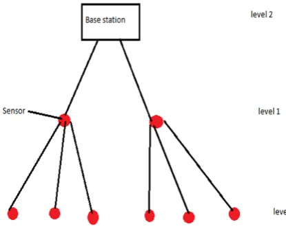
In this, all the nodes are arranged in form of tree structure, in which the intermediate node can perform data aggregation process and transmission of data is performed from leaf node to root node. Tree based topology [5] is basically used in the applications where in network data aggregation is required. In this approach aggregation is performed by constructing an aggregation tree which could be a minimum spanning tree, in which leaf node sends data
to parent node and then after root node. Each node has a parent node to forward it’s data. This is the appropriate method for designing optimal aggregation techniques. E.g. Radiation-level monitoring in nuclear plant.
Figure 2: Tree based data aggregation
Advantages Of Tree Based Data Aggregation:
Ability to tolerate disconnection and loss
Simple in nature.
Easy to implement.
Find the optimal tree with shortest path.
Shorter delay.
2 PROBLEM DEFINITION
Since load balancing in probabilistic wireless sensor network is the major concept of my work, the measurement of the traffic load under the PNM is main goal and also to construct load balanced data aggregation Tree and load balanced data transmission within the probabilistic WSN. Wireless sensor networks offer an increasingly attractive method of data gathering. Data aggregation techniques aim at eliminating redundant data transmission and thus improve the lifetime of the WSN. In WSN, data transmission took place in multi-hop fashion where each node forwards it’s data to the neighbour node which is nearer to root. Data aggregation is the most efficient way to increase the lifetime of the WSN, and also to save the energy consumption of each node
To be specific, I proposed a Load-Balancing under the PNM in three phases.
1. Identify the set of independent nodes.
2. Identify the set of connecting nodes that are used to connect independent and dependent nodes.
3. To find levels of each node related to the root node.
So to construct LBDAT for probabilistic WSN following things are to be considered:
Identify and highlight the nodes that are connected
with Lossy links [3] when constructing a DAT.
The LBDAT construction problem is NP-complete
3 ALGORITHMS
3.1 Algorithm To Identify Independent Nodes
V = Vs U {v0} → Set of nodes on undirected graph G (V, E,
P(E)) |Vs| = n
|V| = n +1
Step 1: Calculate one hop neighborhood for all the nodes
{i.e. N1(vi) ,0 ≤ i ≤ n.} → list of neighboring nodes
Step 2: Calculate node degree of each node
i.e di = | N1(vi)| for ∀vi ∈ V ; 0 ≤ i ≤ n → no of
neighbouring nodes
Step 3: Calculate average degree of the graph G (V, E,
P(E))
i.e. davg =∑
Step 4: Calculate transmission success ratio Lij between
the two node vi and vj, where ∀vj∈N1(vi).
i.e.
for (i=0 ; i ≤ n; i++) {
for (j=0 ; i ≤ | N1(vi)|; j++) {
L[i][j] =
} }
Step5: Calculate potential load (ρi) at each node
ρi = ∑ ∀ vi∈ V ; 0 ≤ i ≤ n
Where, B= Packet size
γi = data receiving rate of each node Vi
Lij =transmission success ratio
Step 6: Calculate average potential load of the graph G (V,
E, P(E))
i.e. ρavg = ∑
Step 7: Obtain the product
xi = | di – davg | * | ρi –ρavg | ∀ vi∈ Vs ; 1≤ i ≤ n
Note: We won’t calculate the product for v0 i.e. for the sink
node as v0 is added to the MIS by default.
Step8: Sort all the nodes by the xi values in increasing
order and the sorted node Ids are stored in A[n].
Step 9: Let wi be the decision variable such that,
Wi = 1 -> Node is a dominator (independent)
Wi = 0 -> Node is not a dominator
All the dominators together form a Maximal Independent set
Initially, set w0 = 1 i.e. root node is consider as member of
MIS by default
Set wi = 0 | ∀ vi∈ Vs ; 1≤ i ≤ n
Step 10: k=0
While k < n do { i=A[k];
set flag =1
foreach(vj ∈ N1(vi) ){
if (wj != 0 ) {
set Flag= 0; Break; }
}
if (flag ==1) then set wi =1;
k= k+1; }
Step 11: Step 10 Multiple times
3.2 Algorithm To Find Connecting Nodes
1. Identify list of black nodes M from previous steps 2. Initialize empty set S of connecting nodes 3. For each v in M
4. for each neighbor n of v 5. for each neighbor n’ of n 6. if (n’ in (M-v) set) then
7. add node n to set S if not present in S
8. break
9. end if 10. end for 11. end for 12. end for
13. sort set S according to degree 14. Identify total node count N
15. Initialize empty set CNS of new connected neighbour nodes
16. Initialize empty set C of new connected nodes 17. For each v in S
18. Reinitialize CNS 19. Reinitialize C 20. For each v’ in S-v 21. add v’ to CNS 22. add v’ to C
23. For each n in N1(v’) 24. add n to CNS
25. if count(CNS) == N then 26. break
27. end if 28. end for
29. if count(CNS) == N then 30. break
31. end for
32. if count(CNS) == N then 33. break
34. end for
35. return C (final connecting nodes)
3.3 Algorithm To Find The Levels Of Node Related To the Root Node
Let M l represent level of black nodes related to the root node V0
Steps:
1. Identify list of black nodes M from previous steps
2. M’=M-V0
3. Set M 0 = V0
4. Find v = set of one hop neighbour of V0 i.e. N1 (V0 )
5. For each node v a. Set VisitedFlag = 1
b. Find z = one hop neighbour of v N1(v)
6. For each node z
a. If node z is present in set M’ b. then
c. Add z to M1
d. Add v to s0
e. Remove z from list M’ f. end if
9. set l =2
10. while (M’ is not empty) i.e. all the black nodes are not covered
a. For each node u in Ml-1
i. Find v = set of one hop neighbour of u i.e. N1 (u)
andhaving VisitedFlag =0 b. For each node v i. Set VisitedFlag = 1
ii. Find z = one hop neighbour of v i.e. N1 (v)
c. For each node z
i. If node z is present in set M’ then ii. Add z to Ml if not present already
iii. add v to Sl-1 iv. end if d. end for e. end for
f. Remove Ml from list M’
11. l ++
12. end while
3. 4 Expected Allocation Probability (EAP):
EAP corresponding to each dominatee (dependent node) and dominator (independent node) pair represents the expected probability that the dominatee is allocated to the dominator. The EAP value associated on each dominatee and dominator pair directly determines the load balance factor of each allocation scheme. I conclude the properties of the EAP values as follows:
1. For each dominate vi , ∑| | 1
where NE(Vi) is the set of neighbouring dominators
of v i , | NE (v i )| is the number of
the nodes in set NE ( v i );
2. In order to produce the most load-balanced allocation scheme, which is obtained when the expected load of allocated dominatees of all the dominators are the same. It can be formulated as follows:
EAPi1 × DL1 = ………… = EAPi|NE(vi)| × DL|NE(vi)|
After calculating EAPij corresponding to each dominatee
and dominator pair, the dominatee vi is allocated to
dominator vj having maximum EAPij value. For the leaf
node vi which is attached to single black node vj EAPij =1
Assign the leaf nodes with EAPij =1
Step 1: For each dominatee vi , find the set of neighbouring
dominators ( black nodes from any level)and store locally (denoted by NE(vi )).
Step 2: For each dominator vi , find the set of neighbouring
dominatees and store locall (denoted by ND (vi )).
Step 3: For each dominator vi , calculate the load DLi
indicates the load at each from its
neighbouring dominates using the formula. DLi = ∑| |
Step 4: If a dominate (dependent, leaf) vi is connected to
only one dominator (independent) vj, the EAP value associated with the pair is equal to 1.
Step 5: For each dominatee vi , calculate the neighbouring
dominators EAPij using the below formula and store locally. EAPij = ∏
Step 6: The dominatee vi is allocated to dominator vj
having maximum EAPij value.
3.4 Notations Used in Algorithm Sr.no Notation Description
1 V0 Root node
2 Vs Set of n nodes { v1, v2, . . .
,vn}
3 V V=Vs ∪ { V0 }
4 E Set of Lossy Links
5 Lij Probability of that node vi can
successfully transmit a packet to node vj
6 N1(vi) 1-Hop neighbourhood.
7 ρi Potential load.
8 M Set of black nodes.
9 Xi Actual load.
10 C Final list of connecting nodes.
11 γi Data receiving rate.
12 di Node degree
13 B No of bits transferred
14 wi Decision variable. (0/1)
15 L Level of node related to root node
16 S List of temporary connecting
nodes
17 EAP Expected Allocation Probability
18 DL Transmission success ratio of
neighbouring node Table: Notations used.
4 RESULT
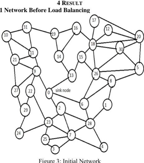
4.1 Network Before Load Balancing
Figure 3: Initial Network
4.2 Network After Load Balancing
Figure 4: Final load balanced network
In the above figure 4
Node 0 is root node and blue colour nodes are the
neighbouring nodes of root node.
Nodes 8, 11, 14, 15, 23, 28 are the level 1 nodes
related to the root node.
Nodes 3, 20 and 29 are the level 2 nodes related to the root node.
Red dotted line indicates the neighbour of level 1 node.
Black dotted line indicates the neighbour of level 2 node.
Nodes 24, 7 and 18 are the intermediate nodes
between level 1 and level 2 nodes.
Nodes 2, 6, 9 and 13 are the intermediate nodes
between level 0 and level 1 nodes.
Level 1 and level 2 nodes are independent nodes that are specifying as Black nodes (As B in figure)
Remaining nodes are dependent nodes that are
specifying as gray nodes (As G in figure)
Above figure shows the final load balanced tree generated by comparing the Expected Allocation Probability (EAP) value of every node. Dotted line indicates the edges for leaf node assignment with maximum EAP.
4.3 Performance Evaluation
Figure 5: Graphical analysis
The graph (Figure 5) showing the graphical analysis of the system in which evaluation result is according to node Vs energy saved by each node. X-axis shows the node ID and Y-axis shows energy-saved by each node.
Here the comparative result is based on the load
balancing with data aggregation and without data aggregation. Red line indicates the analysis with data aggregation and black line indicates analysis without data aggregation. Here we can observe that energy left by each node is more as compare to without data aggregation algorithm. Every node saving near about 30% energy during the transmission. So additionally we can see load balancing with data aggregation prolongs the network life time though there is a saving of energy by each node. Result can demonstrate that the proposed system is near about 40% efficient than the other algorithm.
Figure 6: Hello packet transmission
4.4 Load Balanced Data Transmission
Figure 8: Transmission from node 5 to node 8
Figure 9: Transmission from node 1 to node 8
Fig 10: Transmission from node 26 to node 8
Fig 11: Transmission from node 8 to node 6
Fig 12: Transmission from node 6 to root node
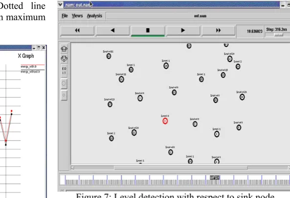
Figure 6 to figure 12 shows the evaluation result of the NAM consol window. In which, figure 6 shows the HELLO packet transmission by each node to every node. Hello packet transmission is used to find the neighbouring nodes of each node.
Figure 7 indicates the level detection of
independent nodes with respect to sink node. Level 1 indicates the 1-hop neighbour node of sink node and level 2 indicates the 1-hop neighbour node of level 1 independent nodes.
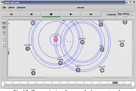
Figure 8 to figure 12 shows the level 1 data
transmission, in which data can be transferred as follows.
Node 5 (leaf node of 8)-> node 8 (Level 1 node)-> node 6 (leaf node of sink node)-> sink node. Node 26 and node 1 also sending data to node 8 as they are also leaf node of 8.
5 CONCLUSIONS
Data aggregation provides energy conservation and also removes redundant data during the transmission and provides required data only. So Tree based data aggregation technique is most suitable to achieve load balancing in wireless senor network. As increase in use of WSN for number of applications, load balancing is the major concern in my proposed system and to use WSN in an efficient manner and also to increase the lifetime of the sensor networks. I have successfully performed the load balancing on probabilistic wireless sensor network. Result shows the load balanced data aggregation tree. After the successful load balancing I have performed the successful communication from leaf node to root node. Level wise communication is performed between the nodes that mean firstly I have performed level 1 transmission and then level 2 transmission.
ACKNOWLEDGEMENT
REFERENCES
[1] S. Ji, J. He, Y. Pan, and Y. Li, ‘‘Continuous Data Aggregation and Capacity in Probabilistic Wireless Sensor Networks,’’ J. Parallel Distributed. Computing, vol. 73, no. 6, pp. 729-745, June 2013. [2] Hwa-chun Lin, Feng-Ju Li and Kai-Yang Wang, “ Constructing
Maximum-lifetime Data gathering Trees in sensor network with Data Aggregation” , IEEE ICC 2010.
[3] A. Cerpa, J. Wong, L. Kuang, M. Potkonjak, and D. Estrin, ‘‘Statistical Model of Lossy Links in Wireless Sensor Networks,’ in Proc. IPSN, 2005, pp. 81-88.
[4] Y. Liu, L.M. Ni, and C. Hu, ‘‘A Generalized Probabilistic Topology Control for Wireless Sensor Networks,’’ IEEE J. Sel. Areas Commun., vol. 30, no. 9, pp. 1780-1788, Oct. 2012
[5] Divya Sharma, Sandeep Verma and Kanika S., “Network Topologies in Wireless Sensor Network: A Review”, IJECT, Vol. 04, pp 93-97, June 2013.
[6] Hwa-chun Lin, Feng-Ju Li and Kai-Yang Wang, “ Constructing Maximum-lifetime Data gathering Trees in sensor network with Data Aggregation” , IEEE ICC 2010.