(will be inserted by the editor)
Solving a Class of Modular Polynomial Equations and its
Relation to Modular Inversion Hidden Number Problem
and Inversive Congruential Generator
Jun Xu · Santanu Sarkar · Lei Hu · Zhangjie Huang · Liqiang Peng
Received: date / Accepted: date
Abstract In this paper we revisit the modular inversion hidden number problem (MIHNP) and the inversive congruential generator (ICG) and consider how to attack them more efficiently. We consider systems of modular polynomial equations of the formaij+bijxi+cijxj+xixj = 0 (modp) and show the relation between solving such equations and attacking MIHNP and ICG. We present three heuristic strategies using Coppersmith’s lattice-based root-finding technique for solving the above modular equations.
In the first strategy, we use the polynomial number of samples and get the same asymptotic bound on attacking ICG proposed in PKC 2012, which is the best result so far. However, exponential number of samples is required in the work of PKC 2012. In the second strategy, a part of polynomials chosen for the involved lattice are linear combinations of some polynomials and this enables us to achieve a larger upper bound for the desired root. Corresponding to the analysis of MIHNP we give an explicit lattice construction of the second attack method proposed by Boneh, Halevi and Howgrave-Graham in Asiacrypt 2001. We provide better bound than that in the work of PKC 2012 for attacking ICG. Moreover, we propose the third strategy in order to give a further improvement in the involved lattice construction in the sense of requiring fewer samples.
Keywords Modular inversion hidden number problem ·inversive congruential generator·lattice·LLL algorithm·Coppersmith’s technique
Mathematics Subject Classification (2000) 94A60
J. Xu·L. Hu·Z. Huang·L. Peng
State Key State Laboratory of Information Security, Institute of Information Engineering, Chinese Academy of Sciences, Beijing 100093, China
Data Assurance and Communication Security Research Center, Chinese Academy of Sciences, Beijing 100093, China
E-mail:{xujun,hulei,huangzhangjie,pengliqiang}@iie.ac.cn
S. Sarkar ()
1 Introduction
1.1 Background
Modular Inversion Hidden Number Problem.Hidden Number Problem (HN-P) was introduced in [6] by Boneh and Venkatesan. They used it to prove that computing the most significant bits (MSBs) of the secret key from the public keys of participants in a Diffie-Hellman key-exchange protocol is as hard as computing the secret key itself. The work [6] has originated a whole direction of research and HNP has been exploited in a wide spectrum of applications like an attack on weak versions of the Digital Signature Algorithm (DSA) [13] and appeared in a number of questions, related and unrelated to cryptography (see [22] for a survey of relevant results and also [1] for some developments in this direction).
A closely related class to HNP, known as Modular Inversion Hidden Num-ber Problem (MIHNP), was introduced and studied in [5] by Boneh, Halevi and Howgrave-Graham. They utilized MIHNP to construct pseudo random number generator (PRNG) and message authentication code (MAC). The exact problem (MIHNP) is as follows.
For a given prime p, consider a secretα∈Zp andn+ 1 elementst0, t1, . . . , tn
∈Zp\{−α}, chosen independently and uniformly at random. The question is, given
n+ 1 samples
ti,MSBδ((α+ti)−1modp)
n
i=0 for someδ >0 (here MSBδ(z)
refers to the δ most significant bits of z), whether it is possible to recover the hidden numberα.
Inversive Congruential Generator.Number-theoretic PRNGs work by iterating an algebraic mapf over a residue ringZN on a secret random initial seed valuev0
to compute valuesvi+1=f(vi) modN. The output is some consecutive bits of the state valuevi at each iteration. The first inputv0 is called the seed. PRNGs have
numerous applications in signature schemes and public key encryption schemes. When f is affine, generator is known as linear congruential generator. However this generator is not cryptographically secure [7, 23]. It was suggested to use a non-linear algebraic mapf in order to avoid these attacks.
The Inversive Congruential Generator (ICG) proposed by Eichenauer and Lehn [10] is an important kind of nonlinear number-theoretic pseudo random number generator. There are extensive applications of ICG in Quasi-Monto Carlo simulation and public key schemes (see the surveys in [11, 16, 17, 19, 24] and recent results in [18, 20, 21, 25]). ICG works as follows:
For a given prime p, let f(x) = ax−1+b (mod p) where a, b ∈ Zp. Input a secret seedv0 to the recursive relation vi+1=f(vi) for 0≤i≤n. Then output a random-looking sequence (MSBδ(v1),MSBδ(v2),· · ·,MSBδ(vn+1)).
A very strong goal of attacking ICG is to recover the secret seedv0givenn+ 1
outputs MSBδ(vi+1) fori= 0,1· · ·, n.
1.2 Previous Works
heuristic (where multiples are used [5, Section 3.2] that we refer here as Method II) claimed knowledge of significantly fewer bits which isδ > 13log2ponly. However, no explicit lattice construction for this case was presented.
Ling et al. [15] provided a rigorous probabilistic polynomial time algorithm for MIHNP. The work in [15] could match one of the heuristics (Method I) of Boneh et al. [5], where one requires two-third of the bits of the output to solve the problem. However, Ling et al. could not theoretically justify the more efficient heuristic (Method II) by Boneh et al., that requires only one-third of the bits of the output.
Based on the observation that the algorithm in [15] is not ideal when the num-ber of samples is relatively small, Xu et al. [26] proposed a heuristic lattice method by combining Coppersmith’s lattice technique and the priority queue technique. The corresponding result isδ > 12log2p, which is better than that of Method I of
Boneh et al in [5] and the rigorous algorithm of Ling et al. in [15], but weaker than Method II of Boneh et al.
Attack of ICG.In [3,4], Blackburn et al. pointed out that ICG can be attacked in polynomial time if sufficiently many bits of some consecutive valuesviare revealed by combining lattice method and linearization technique. In PKC 2012, Bauer et al. [2] improved the work of Blackburn et al. by utilizing Coppersmith’s method. They showed that the secret seed of ICG can be recovered if more than 12 portion of most significant bits ofvi’s are given, i.e.,δ > 12log2p, provided that the number
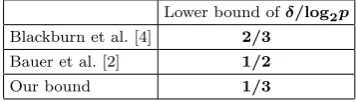
of samples is sufficiently large. In this paper, we improve the bound ofδ. In Table 1, we compare new bound ofδ with the existing bounds for ICG.
Table 1 Comparison of asymptotic lower bound ofδfor ICG with existing methods.
Lower bound ofδ/log2p
Blackburn et al. [4] 2/3
Bauer et al. [2] 1/2
Our bound 1/3
1.3 Our Contribution
We first translate the recovering problem of the hidden number in MIHNP and the secret seed of ICG into solving multivariate modular polynomial equations
aij+bijxi+cijxj+xixj= 0 (modp),0≤i < j≤n
and then, we give three heuristic lattice methods to find the small solutions of the above modular equations.
In the first strategy, for given n+ 1 samples in MIHNP or n+ 1 outputs in ICG, the hidden number or the secret seed can be recovered when the number of known MSBs
δ > 1 2+
1 2n+ 2
The asymptotic bound whenn→+∞is better than the first result of Boneh et al. in [5] and the rigorous result of Ling et al. in [15], and same as the asymptotic results in [2, 26]. However, the dimension of the lattices in our first strategy is polynomial onnbut the dimension of the involved lattices in [2, 26] is exponential onn.
In the second strategy, a part of polynomials used for the lattices are linear combinations of several polynomials, which obtains a larger upper bound for the desired root. Givenn+ 1 samples in MIHNP orn+ 1 outputs in ICG, the hidden number or the secret seed can be obtained when
δ >(1−F(n, d))·log2p
where F(n, d) is defined in Section 5 and parameter d satisfies 1 ≤ d ≤ n. For integersnandd, there is always δ
log2p > 1
3. Takingd=c·nfor 0< c≤ 1
2, one can
get
δ log2p
→ 1
3 whenn→+∞.
This asymptotic bound is superior than the best work on the attack of ICG [26] and is same as the result of MIHNP in Method II [5]. However, here we explicitly present lattice construction not given in Method II [5].
In the third strategy, we improve the lattice construction in the second strategy. Under the situation thatn+ 1 samples in MIHNP or n+ 1 outputs in ICG are given, one can get the hidden number or the secret seed if
δ >(1−F(n, d, k))·log2p
where F(n, d, k) is described in Section 6 and 1≤d≤n andk ≥1. For integers n, d, k, there is also always logδ
2p > 1
3. Whenk= 1, it becomes the second strategy.
Whenk > 1, it is better than the second strategy as logδ
2p is closer to 1 3 in this
strategy. Moreover, logδ 2p <
1
2 forn= 4, which is superior to the asymptotic results
in the case that sufficiently many samples are given in [2, 26].
1.4 Organization of the Paper
The rest of this paper is organized as follows. In Section 2, we recall some termi-nologies and preliminary knowledge. In Section 3, we transform analysis of MIHNP and attack of ICG into solving a class of modular polynomial equations. In Sections 4, 5 and 6, we respectively present three strategies for solving a class of modu-lar polynomial equations and give the corresponding applications for MIHNP and ICG. Section 7 is the conclusion.
2 Preliminaries
Throughout the paper, the set {0,1,· · ·, ps−1} is denoted as Zps where s is
some positive integer, in case of need, the elements ofZps are also treated as the
2.1 Order of Monomials
First, we describe reverse lexicographic order and graded lexicographic reverse order respectively. For more details about the orders of monomials, please refer to [9]. Let integer vectorsIn =(i1,· · ·, in),Jn =(j1,· · ·, jn).
Reverse Lexicographic Order:
In≺revlexJn⇔ the rightmost nonzero entry inIn−Jn is negative. For example,
(0,0)≺revlex(3,0)≺revlex(1,1)≺revlex(0,2).
Graded Reverse Lexicographic Order:
In≺grevlexJn⇔ n
X
m=1
im< n
X
m=1
jmor ( n
X
m=1
im= n
X
m=1
jmandIn≺revlexJn).
For vectors in the above example, we have
(0,0)≺grevlex(1,1)≺grevlex(0,2)≺grevlex(3,0).
Next, we define an order of monomials which will be used to arrange the poly-nomials according to their leading mopoly-nomials in the following lattice construction.
A New Defined Order: xi00xi11 · · ·xin
n ≺xj00x j1 1 · · ·x
jn
n ⇔In≺grelexJn or (In=Jn andi0< j0). (1)
For example,f(x0, x1) =a+bx0+cx1+x0x1. According to (1), there is 1≺x0≺
x1≺x0x1. Thus,x0x1 is the leading monomial off(x0, x1).
2.2 Polynomial Coefficients
For positive integers k andn, the coefficient ofxs in the expansion of the poly-nomial (1 +x+· · ·+xk)n is called the polynomial coefficient (ns)k+1, 0≤s≤nk. Namely, we have
(1 +x+· · ·+xk)n= nk
X
s=0
n s
!
k+1
xs,
where (ns)k+1 = P
n1+···+knk=s
(n−n1−···−nn
k,n1,···,nk). Obviously, when k = 1, the
polynomial coefficient (ns)k+1 is the binomial coefficient (ns). Whenm(k+ 1)≤s≤ (m+ 1)(k+ 1)−1, we have
n s
!
k+1
= m
X
i=0
(−1)i n+s−i(k+ 1)−1 s−i(k+ 1)
!
n i
!
,
2.3 Lattice
Let the vectorsb1, . . . ,bω be linearly independent inRn, the set
L=
ω
X
i=1
kibi, ki∈Z
is called a lattice with basis vectors b1,· · ·,bω. The dimension and determinant ofLare respectively
dim(L) =ω,det(L) =
q
det(BBT).
Here,B= [bT1,· · ·,bTω]T is a basis matrix. IfB is a square matrix, then det(L) =
|det(B)|. In this paper all lattice basis matrices are square.
It is well known that the LLL algorithm [14] can find a reduced basis of the lattice as follows.
Lemma 1 ( [14]) Let L be a lattice. Within polynomial time, the LLL algorithm outputs reduced basis vectorsv1, . . . ,vω that satisfy
kv1k ≤ kv2k ≤ · · · ≤ kvik ≤2
ω(ω−1)
4(ω+1−i)det(L) 1
ω+1−i,1≤i≤ω.
2.4 Coppersmith’s Technique
The Coppersmith technique can be used for finding the small solution of modular polynomials. Its key step is to generate more modular polynomials with common root which is the desired solution and then use the lattice reduction algorithms to obtain integer polynomials with the desired root. In this step, the following Lemma reformulated by Howgrave-Graham is needed.
Lemma 2 ( [12]) Letf(x0, x1, . . . , xn) be an integer polynomial that consists of at mostω monomials. Letd be a positive integer and the Xi be the upper bound of|xi| fori= 0,1,· · ·, n. Suppose that
1. f(x0, x1, . . . , xn) = 0 (modpd), 2. kf(x0X0, x1X1, . . . , xnXn)k< p
d √
ω,
thenf(x0, x1, . . . , xn) = 0holds overZ.
Now see thatkf(x0X0, x1X1, . . . , xnXn)kin Lemma 2 is the Euclidean norm of the coefficient vector of the polynomialf(x0X0, x1X1, . . . , xnXn). This is also the norm of the corresponding row vector of the involved lattice. To obtain at least n+ 1 polynomials with the common desired root (x0, x1, . . . , xn), from Lemma 1 and Lemma 2, we need
2ω (ω−1)
4(ω−n) ·(det(L)) 1
ω−n < p
d
√
ω (2)
Since the terms 2ω (ω−1)
4(ω−n) and√ω are much smaller than p, we give the following simplified condition
whereω= dim(L). Further, we expect that the obtained integer polynomials are algebraically independent. Then, we can utilize numerical or symbolic methods such as the resultant method or the Gr¨obner basis technique to compute the desired root (x0, x1, . . . , xn). In this process, the following assumption is used.
Assumption 1. Let g1,· · ·, gn+1 ∈ Z[x0, x1,· · ·, xn] be the polynomials that are found by Coppersmith’s technique. Then the ideal generated by the polynomial equations g1(x0, x1,· · ·, xn) = 0,· · ·,gn+1(x0, x1,· · ·, xn) = 0has dimension zero.
We consider the above assumption to be true in all the results that will be presented in this paper. In all the experiments, we observe the correctness of the assumption. So we collect the roots efficiently using Gr¨obner basis technique.
We implement programs in SAGE 5.13 on a Linux Mint 12 on a laptop with Intel(R) Core(TM) i5-4200U CPU @ 1.60GHz, 3 GB RAM and 3 MB Cache.
3 A Class of Modular Polynomial Equations
In this section, we obtain a class of modular polynomial equations with small roots from the analysis of HIMNP and the attack on ICG respectively.
3.1 Analysis of MIHNP
First, we propose the following problem on the analysis of MIHNP.
Problem 1 For a sufficiently large primep, consider a hidden numberα∈Zpand
n+ 1 elementst0, t1, . . . , tn ∈Zp\ {−α}, chosen independently and uniformly at random. The goal is to recoverαgivenn+ 1 samples
ti,MSBδ((α+ti)−1modp)
n
i=0
for somek >0.
Next, we transform Problem 1 into solving simultaneous modular equations with small roots. Since the MSBδ((α+ti)−1modp)) (i.e., δ many MSBs of the integers (α+ti)−1modp) are known, we let ui = MSBδ((α+ti)−1modp)) and can write ui+xi = (α+ti)−1modp where ui is known and xi is unknown for
i= 0,1,· · ·, n. Rearranging the above relations, we get (α+ti)(ui+xi) = 1 (modp).
Further, eliminatingαfrom these equations, we can obtain (n+12 ) modular equa-tions as follows:
aij+bijxi+cijxj+xixj = 0 (modp),0≤i < j≤n, (3) where
aij=uiuj+ (ui−uj)(ti−tj)−1modp,
bij=uj+ (ti−tj)−1modp,
cij=ui−(ti−tj)−1modp.
Since δ many MSBs of (α+ti)−1modp are known, we have 0 ≤ xi ≤ 2pδ for
3.2 Recovering Seed Attack on ICG
First, let us recall ICG. For a given prime p, the generator function of ICG is f(x) =ax−1+b(mod p) where a, b∈Zp. Input a secret seed v0 to the recursive
relationvi+1 =f(vi) for 0≤i≤n. Then outputs are MSBδ(vi+1) (i.e.,δ many
MSBs ofvi+1) for someδ >0. Naturally, one concerns with the attack on recovering
the secret seed. In other words, one will consider the following concrete problem.
Problem 2 For a sufficiently large primep, the goal is to recover the seedv0given
n+ 1 ICG outputs
MSBδ(vi+1) n i=0.
Then, let us translate Problem 2 into finding small roots of modular equations. According to the relationsvi+1=av−1i +b(mod p) for 0≤i≤n, we have
a+bvi−vivi+1= 0 modp, i= 0,1,· · ·, n.
From these relations, we can use the resultant method and generate relations a0ij+b0ijvi+c0ijvj+d0ijvivj= 0 modpfor 0≤i < j≤n+ 1, (4) where a0ij, b0ij, c0ij, dij0 are known. For example we have a+bv1−v1v2 = 0 modp
anda+bv2−v2v3 = 0 modp. Now we utilize the resultant method to eliminate
the variablev2and get
ab+ (a+b2)v1−av3−bv1v3= 0 modp.
Next, letui+1= MSBδ(vi+1), we can write
vi+1=ui+1+xi fori= 0,1,· · ·, n (5) where ui+1 is known and xi is unknown. Now plugging (5) into the relations in (4), we get the following relations
aij+bijxi+cijxj+xixj = 0 modpfor 0≤i < j≤n (6) where the integersaij, bij, cij are known. Sinceδ many MSBs ofvi are known, we get 0≤xi≤ 2pδ for 0≤i≤n. Obviously, ifxi’s are found out, we can recover the
seedv0 from (4) and (5).
Note that the forms of equations in (3) and (6) are the same. Therefore, in order to solve Problems 1 and 2, our goal in the following sequel is to find the small roots (xi, xj) of the following modular polynomial equations
fij(xi, xj) :=aij+bijxi+cijxj+xixj= 0 (modp),0≤i < j≤n (7) wherex0, x1,· · ·, xn are bounded byX. In the cases of MIHNP and ICG, we take
X= 2pδ whereδ is the number of known MSBs.
Assumption 2. Assume that thec0,j in equation (7) are independent and uniformly random inZp for allj= 1,· · ·, nand positive number n
2
p is negligible.
Based on Assumption 2, we can deduce that the c0,j are distinct inZp for all
j= 1,· · ·, nwith overwhelming probability. Concretely speaking, from thec0,j are independent and uniformly random inZpfor allj= 1,· · ·, n, we have
Pr{all c0,j are distinct mod p f or j= 1,· · ·, n}= n−1
Y
i=1
(1− i p).
Note that n2
p is negligible, we get n−1
Y
i=1
(1− i p)≈e
−n− 1 P
i=1
i p
=e−
n(n−1)
2p ≈1−n 2−n
2p ,
which is close to 1.
4 The First Strategy on Solving (7)
In this section, we propose the first strategy for solving (7) and give the corre-sponding application on MIHNP and ICG. First, we present the following heuristic result, which is verified by our experiments.
Result 1. For given polynomials fij(xi, xj) with 0 ≤ i < j ≤n in (7), under As-sumption 1, one can solve (7) in time polynomial in(n,logp)when the bound X of x0, x1,· · ·, xn satisfies
X < p12− 1 2n+2−1
where1is some positive real number.
Proof. Consider the following set of polynomials
P=
p, px0, px1,· · ·, pxn, f0,1,· · ·, f0,n,· · ·, fn−1,n
.
Now construct a latticeLusing the coefficient vectors ofh(x0X, x1X, . . . , xnX) for eachh∈ P.
Then the matrixM, corresponding toL, is of the form
x0x1 . . . x0xn . . . xn−1xn x0 . . . xn 1
X2 . . . 0 . . . 0 − . . . 0 −
..
. . .. ... ... ... ... . .. ... ...
0 . . . X2 . . . 0 − . . . − −
..
. ... ... . .. ... ... . .. ... ...
0 . . . 0 . . . X2 0 . . . − −
0 . . . 0 . . . 0 Xp . . . 0 0
..
. ... ... ... ... ... . .. ... ...
0 . . . 0 . . . 0 0 . . . Xp 0
0 . . . 0 . . . 0 0 . . . 0 p
Here ‘−’ indicates non zero element.
Clearly, the dimension of Lis dim(L) = (n+12 ) +n+ 2. Also
det(L) =pn+2·
n+1 z }| {
X· · ·X· (n+1
2 )
z }| {
X2· · ·X2=pn+2X(n+1)2.
By the property of LLL algorithm and Howgrave-Graham’s lemma, if the condition (2) satisfies (hered= 1), i.e., there is
ωω −n
2 2
ω(ω−1) 4 pn
·det(L)< pω (8)
whereω= det(L), after reduction of lattice we getn+ 1 polynomialsg1,· · ·, gn+1
which contain the root (x0, x1,· · ·, xn) over integers. Under Assumption 1, we can findx0, x1,· · ·, xn fromg1,· · ·, gn+1.
Finally, we analyze the situation that the condition (8) holds. Plugging the determinant and dimension of the latticeLinto (8), we get the condition
X <
ωω −n
2 2
ω(ω−1) 4 pn
−(n+1)21
·p12− 1 2n+2.
Note thatω= (n+12 ) +n+ 2<(n+ 1)2for n >2, we can deduce that
ωω−2n2
ω(ω−1) 4 pn
(n+1)21
< ω122
ω−1 4 p
n
(n+1)2 =p1
where1= 2 log4 log2ω+(ω−1) 2p +
n
(n+1)2 >0. It implies that the right side of the above condition on X can be lower bounded byp12−
1
2n+2−1. Hence, in order to let (8) be satisfy, we need
X < p12− 1 2n+2−1.
When log2pdim(L) andnis large enough,1is negligible.
Note that X = 2pδ for the situations of MIHNP and ICG. Hence, we have the
following application.
Application 1. Given n+ 1 samples in MIHNP or n+ 1 outputs in ICG, under Assumption 1, one can recover the hidden number or the secret seed in time polynomial in(n,log2p)if the numberδ of known MSBs satisfies
δ log2p>
1 2 +
1
2n+ 2+1.
Remark 1 It is shown that one can obtain the hidden number in MIHNP if logδ 2p > 2
3 for n→ ∞ by using the first heuristic method in [5] or the rigorous technique
in [15] respectively. In this section, we need logδ 2p >
1
2 forn→ ∞. Hence, we get
the better heuristic bound.
Remark 2 It is proved that one can heuristically recover the hidden number in MIHNP [26] or the secret seed in ICG [2] if logδ
2p > 1
2 for n → ∞ using the
Remark 3 The asymptotic result of the first strategy is better than those of the Method I in [5] or the rigorous technique in [15], which is due to that it uses all basic polynomials fij(xi, xj) with 0≤i < j≤n. Although the first strategy gets the same asymptotic result as [2, 26] when n → ∞, it obtains worse bounds for givenn, which is because that it only utilizes all basic polynomials instead of their shifts or powers. We present the concrete comparison in Table 4.
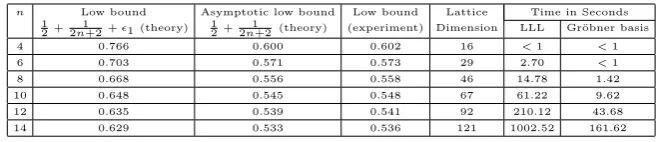
Experimental results. The first strategy works successfully with low lattice di-mensions and we can easily obtain the experimental results for a few values of n ≤ 14 as given in Table 2. In our experiments, we find out that the condition det(L)< pω−o(1)is sufficient for the attack in the first strategy.
Table 2 Experimental results of the first strategy on low bounds oflogδ
2p for 1000-bitp.
n Low bound Asymptotic low bound Low bound Lattice Time in Seconds 1
2+2n1+2+1 (theory) 12+2n1+2(theory) (experiment) Dimension LLL Gr¨obner basis
4 0.766 0.600 0.602 16 <1 <1
6 0.703 0.571 0.573 29 2.70 <1
8 0.668 0.556 0.558 46 14.78 1.42
10 0.648 0.545 0.548 67 61.22 9.62
12 0.635 0.539 0.541 92 210.12 43.68
14 0.629 0.533 0.536 121 1002.52 161.62
5 The Second Strategy on Solving (7)
In this section, we give the second strategy on Solving (7) and use it to analyze MIHNP and ICG. First, let us define the notation
F(n, d) =
2d
d
P
s=0
s(ns)
d(d+ 1) d
P
s=0
(ns) + 2(d+ 1) d
P
s=0
s(ns)
and the set
I(n, d) ={(i0, i1,· · ·, in)|0≤i0≤d,0≤i1,· · ·, in≤1,0≤i1+· · ·+in≤d}
where integers n, d satisfy 0 ≤ d ≤ n. Then, we propose the following heuristic result, which is also confirmed by our experiments.
Result 2. For given polynomialsf0j(x0, xj)with1≤j≤nin (7), under Assumptions 1 and 2, one can solve (7) in polynomial time, if the boundX ofx0, x1,· · ·, xn satisfies
X < pF(n,d)−2
Proof. First, we construct the polynomialfi0,i1,...,in(x0, x1,· · ·, xn) such that the
leading monomial isxi00xi11 · · ·xin
n in terms of the defined order (1), where the tuples (i0, i1,· · ·, in)∈I(n, d).
Case 1:Wheni1+· · ·+in= 0, we havei1=· · ·=in= 0 andxi00xi11 · · ·xinn=xi00.
We generate the polynomial
fi0,i1,...,in(x0, x1,· · ·, xn) =x
i0
0. (9)
Clearly,xi00xi11 · · ·xin
n is the corresponding leading monomial.
Case 2:Wheni1+· · ·+in≥1, lets=i1+· · ·+in, we can write
xi00xi11 · · ·xin
n =xi00 ·(xj1· · ·xjs)
where 1≤s≤dand 1≤j1<· · ·< js≤n. For example,
x20x11x02x13x41=x20·(x1x3x4).
Here n = 4, s = 3, and xj1 = x1, xj2 = x3, xj3 = x4. Then, we construct the
polynomialfi0,i1,...,in according to the following two situations:
Case 2.a:Fori0≥s, we generate the polynomial
fi0,i1,...,in(x0, x1,· · ·, xn) =x
i0−s
0 f0,j1· · ·f0,js. (10)
It is easy to see thatfi0,i1,...,in(x0, x1,· · ·, xn) = 0 modp
sandxi0 0x
i1 1 · · ·x
in
n is the leading monomial in this case.
Case 2.b:For 0≤i0< s, consider the polynomials
gl(x0, xj1,· · ·, xjs) = (f0,j1· · ·f0,jl−1)·xjl·(f0,jl+1· · ·f0,js) forl= 1, . . . , s.
It is easy to see that gl(x0, xj1,· · ·, xjs) = 0 modp
s−1 for l= 1, . . . , s. Note that
the polynomialsg1,· · ·, gs have common monomials
xj1· · ·xjs, x0·(xj1· · ·xjs),· · ·, x
s−1
0 ·(xj1· · ·xjs).
We can rewrite the polynomialsg1,· · ·, gsaccording to the following way:
g1 g2 .. . gs
=M[j1,· · ·, js]·
xj1· · ·xjs
x0xj1· · ·xjs
.. . xs0−1xj1· · ·xjs
+ h1 h2 .. . hs . (11)
Here, the polynomialhl (1≤l≤s) is composed of the terms ingl except for the corresponding terms of the above common monomials and the matrix
M[j1,· · ·, js] =
σs−1(∧1)· · · σ1(∧1) 1
σs−1(∧2)· · · σ1(∧2) 1
· · ·
σs−1(∧s)· · · σ1(∧s) 1
whereσi(∧l) is thei-th elementary symmetric polynomial on
∧l:= (c0,j1,· · ·, c0,jl−1, c0,jl+1,· · ·, c0,js)
with 1≤i≤s−1 and 1≤l≤s. Let us continue with the monomialx02x11x02x13x14.
We first construct
g1=x1·(f0,3f0,4), g2=x3·(f0,1f0,4), g3=x4·(f0,1f0,3),
which have common monomialsx1x3x4, x0x1x3x4, x20x1x3x4. Then, we get g1 g2 g3 =
c0,3c0,4 c0,3+c0,4 1
c0,1c0,4 c0,1+c0,4 1
c0,1c0,3 c0,1+c0,3 1
x1x3x4
x0x1x3x4
x20x1x3x4 + h1 h2 h3 .
We can compute out the determinant of the matrix M[j1,· · ·, js] by mathe-matical induction, i.e.,
det(M[j1,· · ·, js]) =
Y
1≤l<t≤s
(c0,jl−c0,jt).
Under Assumption 2, we have obtained that all c0,j are distinct in Zp for j = 1,· · ·, n with overwhelming probability. Then, det(M[j1,· · ·, js]) is coprime to primepand hence any power ofp, and the inverse ofM[j1,· · ·, js] exists mod the power ofp. Let integer matrixU[j1,· · ·, js] be the inverse of matrixM[j1,· · ·, js] modps−1, i.e.,
U[j1,· · ·, js]·M[j1,· · ·, js] =Is (modps−1).
Multiplying (11) by U[j1,· · ·, js] from the left and taking modulo ps−1 on both sides, we get
U[j1,· · ·, js]·
g1 g2 .. . gs ≡
xj1· · ·xjs
x0xj1· · ·xjs
.. . xs0−1xj1· · ·xjs
+U[j1,· · ·, js]·
h1 h2 .. . hs
(modps−1). (12)
Let (ui0+1,1,· · ·, ui0+1,s) be the (i0+ 1)-th row of U[j1,· · ·, js], where 0≤ i0 ≤
s−1. Then, we form the polynomial
fi0,i1,...,in(x0, x1,· · ·, xn) =ui0+1,1·g1+· · ·+ui0+1,s·gs. (13)
Since thatgl(x0, x1,· · ·, xn) = 0 modps−1for all 1≤l≤s, there is
fi0,i1,...,in(x0, x1, . . . , xn) = 0 modp
s−1
.
Moreover, the leading monomial of fi0,i1,...,in(x0, x1,· · ·, xn) in this situation is
alsoxi00xi11 · · ·xin
Next, we utilize the idea of Coppersmith’s technique and construct the lattice L(n, d) using the coefficient vectors of the polynomialshi0,i1,···,in(x0, x1,· · ·, xn)
=
pd·fi0,i1,...,in(x0X0, x1X1,· · ·, xnXn) Case 1
pd−s·fi0,i1,...,in(x0X0, x1X1,· · ·, xnXn) Case 2.a
pd+1−s·fi0,i1,...,in(x0X0, x1X1,· · ·, xnXn) Case 2.b
wheres=i1+· · ·+in. Obviously, for all tuples (i0, i1,· · ·, in)∈I(n, d), there are
hi0,i1,···,in(x0, x1,· · ·, xn) = 0 modp
d
.
We arrange these polynomials according to the leading monomials and can make the corresponding basis matrix be a lower triangular. It is easy to see that the dimension ofL(n, d) is equal to the number of vectors inI(n, d), i.e.,
dim(L(n, d)) = (d+ 1) d
X
s=0
n s
!
. (14)
We can compute the determinant ofL(n, d) as
det(L(n, d)) =pα(n,d)·Xβ(n,d), (15) where
α(n, d) =d(d+ 1) d
X
s=0
n s
!
−d
d
X
s=0
s n s
!
and
β(n, d) =d(d+ 1) 2
d
X
s=0
n s
!
+ (d+ 1) d
X
s=0
s n s
!
.
The detail computation is left in Appendix B. By the property of LLL algorithm and Howgrave-Graham’s lemma, if the condition (2) satisfies, namely,
ωω−2n2
ω(ω−1) 4 pdn
·det(L(n, d))< pdω (16)
where ω= dimL(n, d), after reduction of lattice we get n+ 1 polynomials which contain the root (x0, x1,· · ·, xn) over integers. Under Assumption 1, we can find
x0, x1,· · ·, xn.
Finally, we analyze the case that (16) holds. Plugging (14) and (15) into (16), we obtain the condition
X <
ωω−2n2
ω(ω−1) 4 pdn
−β(n,d1 )
·p
dω−α(n,d)
β(n,d) .
The right side of this condition can be lower bounded bypF(n,d)−2 where 2 = 2 log2ω+(ω−1)
2(d+2) log2p + dn
β(n,d)>0. The detail analysis is given in Appendix C. Therefore,
in order to make (16) hold, we need
X < pF(n,d)−2.
Since X = 2pδ about the cases of MIHNP and ICG, we give the following
application.
Application 2. Given n+ 1 samples in MIHNP or n+ 1 outputs in ICG, under Assumptions 1 and 2, we can recover the hidden number or the secret seed in polynomial time when the numberδof known MSBs satisfies
δ
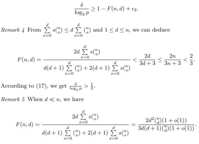
log2p≥1−F(n, d) +2. (17)
Remark 4 From d
P
s=0
s(ns)≤d d
P
s=0
(ns) and 1≤d≤n, we can deduce
F(n, d) =
2d
d
P
s=0
s(ns)
d(d+ 1) d
P
s=0
(ns) + 2(d+ 1) d
P
s=0
s(ns) < 2d
3d+ 3≤ 2n 3n+ 3<
2 3.
According to (17), we get logδ 2p >
1 3.
Remark 5 Whendn, we have
F(n, d) =
2d
d
P
s=0
s(ns)
d(d+ 1) d
P
s=0
(ns) + 2(d+ 1) d
P
s=0
s(ns)
= 2d
2(n
d)(1 +o(1)) 3d(d+ 1)(nd)(1 +o(1)).
Takingd=c·nwhere 0< c≤1
2, there isF(n, d)→ 2
3 whenn→+∞. According to
(17), we have logδ 2p →
1
3. This asymptotic result is better than those in [2, 15, 26],
the first result of Boneh et al. in [5] and the result of the first strategy in Section 4, and same as the second result in [5], which however did not give an explicit lattice construction.
Experimental results.The second strategy works efficiently with low lattice di-mensions and we present our experimental results given in Table 3. In these ex-periments, we observe that the condition det(L(n, d))< pd·dim(L(n,d))is sufficient to find the desired solutions with an exception where (n, d) = (3,2). We can see that the experiment values are better than the corresponding theoretical results in most cases.
Table 3 Experimental results of the second strategy on low bounds oflogδ
2p for 1000-bitp.
n d Low bound Asymptotic low bound Low bound Lattice Time in Seconds 1−F(n, d) +2 (theory) 1−F(n, d) (theory) (experiment) Dimension LLL Gr¨obner basis
3 2 0.754 0.625 0.630 21 <1 <1
4 3 0.651 0.585 0.555 60 29.57 <1
5 3 0.613 0.562 0.525 104 1105.61 14.29
6 3 0.594 0.548 0.505 168 11742.05 149.82
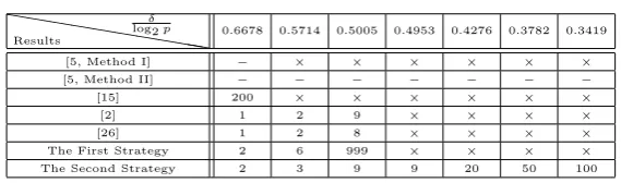
Comparison.In Table 4 and Table 5, we compare the result between the second strategy and the existing works. The symbols “−” and “×” respectively denote that the concrete result was not given and the concrete situation can not be reached in the corresponding paper. In Table 4, we compute the needed minimum value of the ratio logδ
2p for the fixedn. In Table 5, we present the needed smallestnfor the fixed logδ
2p. The correspondingdis optimal in our second strategy. Forn≥9, we can see that the ratiologδ
2p <1/2, which is better than the results in [2,15,26], the first work in [5] and the result in the first strategy. Interestingly, the ratio logδ
2p in our result is close to 1
3 whenn≥100.
Table 4 The minimum value of δ
log2pfor fixedn
````
``
Results
n
1 2 3 4 5 6 7 8 9
[5] - - -
-[2] 0.6667 0.5714 0.5333 0.5161 0.5079 0.5039 0.5020 0.5010 0.5005 [15] 0.8889 0.7778 0.7407 0.7222 0.7111 0.7037 0.6984 0.6944 0.6914 [26] 0.6667 0.5417 0.5083 0.5014 0.5002 0.5000 0.5000 0.5000 0.5000
The First Strategy 0.7500 0.6667 0.6250 0.6000 0.5833 0.5714 0.5625 0.5556 0.5500
The Second Strategy 0.7500 0.6667 0.6250 0.5841 0.5611 0.5378 0.5220 0.5073 0.4953
d= 1 d= 2 d= 2,3 d= 3 d= 3 d= 4 d= 4 d= 5 d= 5
Table 5 The smallestnneeded for fixed logδ
2p
hhhhhh
hhhh
Results
δ
log2p 0.6678 0.5714 0.5005 0.4953 0.4276 0.3782 0.3419
[5, Method I] − × × × × × ×
[5, Method II] − − − − − − −
[15] 200 × × × × × ×
[2] 1 2 9 × × × ×
[26] 1 2 8 × × × ×
The First Strategy 2 6 999 × × × ×
The Second Strategy 2 3 9 9 20 50 100
6 The Third Strategy on Solving (7)
In this section, we give the third strategy for solving (7) and present further improvement on analyzing MIHNP and ICG. First, let us define notations
F(n, d, k) =
(2dk+1) dk
P
s=0 s(n
s)k+1−n
k
P
i=0
min{dk−i,(n−1)k} P
s=0
i2(n−1
s )k+1 (dk+1)dkPdk
s=0(
n
s)k+1+2(dk+1)
dk
P
s=0 s(ns)
k+1
,
andI(n, d, k) =
where integers n, d, k satisfy 0 ≤ d ≤n andk ≥ 1. Then, we give the following heuristic result, which is also certified by the corresponding experiments.
Result 3. For given polynomialsf0j(x0, xj)with1≤j≤nin (7), under Assumptions 1 and 2, one can solve (7) in polynomial time, if the boundX ofx0, x1,· · ·, xn satisfies
X < pF(n,d,k)−3
where3is some positive real number.
Proof. First, we generate the polynomialfi0,i1,···,in(x0, x1,· · ·, xn) such that the
leading monomial is xi00xi11 · · ·xin
n in terms of the defined order (1), where all (i0, i1,· · ·, in) ∈ I(n, d, k). Let m = max{i1,· · ·, in}, we discuss the following t-wo situations in accordance withm.
Case 1:Whenm= 0, we havei1=· · ·=in= 0. In this case, we generate
fi0,i1,···,in(x0, x1,· · ·, xn) =x
i0 0.
Case 2: Whenm > 0, we classify variables x1,· · ·, xn in monomial xi00x i1 1 · · ·x
in
n according to their exponents. Let 1≤s1≤s2≤ · · · ≤sm≤nand
{xj1,· · ·, xjs1} ⊆ {xj1,· · ·, xjs2} ⊆ · · · ⊆ {xj1,· · ·, xjsm} ⊆ {x1,· · ·, xn}
where the corresponding exponents of the variables in{xj1,· · ·, xjst}are greater than or equal to (m−t+ 1) fort= 1,2,· · ·, m. Thus, we can rewrite
xi00xi11 · · ·xin
n =xi00 ·(xj1· · ·xjs1)·(xj1· · ·xjs2)· · ·(xj1· · ·xjsm). (18)
It is easy to see thati1+· · ·+in=s1+· · ·+sm. For example,
x40x21x32x34=x40·x3·(x3x2)·(x3x2x1)·(x3x2x1).
Heren= 3,m= 4,s1= 1,s2= 2,s3=s4= 3 andxj1 =x3,xj2=x2,xj3=x1.
Case 2.a:Fori0≥(s1+· · ·+sm), we generatefi0,i1,...,in(x0, x1,· · ·, xn) which is
equal to
xi0−(s1+···+sm)
0 ·(f0,j1· · ·f0,js1)·(f0,j1· · ·f0,js2)· · ·(f0,j1· · ·f0,jsm).
It is easy to deduce thatfi0,i1,...,in(x0, x1,· · ·, xn) = 0 modp
i1+···+in due toi 1+
· · ·+in=s1+· · ·+smandxi00xi11 · · ·xinnis the leading monomial of the polynomial
fi0,i1,...,in(x0, x1,· · ·, xn) from (18).
Case 2.b: For i0 <(s1+· · ·+sm), for the sake of analysis, define the variable setSt={xj1,· · ·, xjst}and introduce the new notationg(xi0;St) which is a poly-nomial generated by the second strategy such thatxi0·(xj1· · ·xjst) is the leading monomial fort= 1,· · ·, m.
When the integer l satisfies (s1+· · ·+sl)≤i0<(s1+· · ·+sl+sl+1) where
0≤l≤m−1, we construct the polynomialfi0,i1,...,in(x0, x1,· · ·, xn) as follows:
g(xs10 ;S1)· · ·g(xs0l;Sl)
·g(xi0−(s1+···+sl)
Let us consider the monomialx40x21x32x43. Then we have
S1={x3}, S2={x2, x3}, S3=S4={x1, x2, x3}.
Note that (s1+s2)< i0= 4<(s1+s2+s3), thusl= 2 in this example. Then, we
construct the polynomial
f3,2,3,4(x0, x1, x2, x3) :=g(x10;S1)·g(x20;S2)·g(x10;S3)·g(x00;S4).
In this situation, the leading monomial of the polynomial in (19) is xi00xi11 · · ·xin
n andfi0,i1,...,in(x0, x1,· · ·, xn) = 0 modp
(i1+···+in)−(m−l). The corresponding
anal-ysis is given in Appendix D.
Next, we construct a lattice L(n, d, k) using coefficient vectors of the polyno-mialshi0,i1,...,in(x0, x1,· · ·, xn) which are respectively equal to
pdk·fi0,i1,...,in(x0X0, x1X1,· · ·, xnXn) Case 1
pdk−(i1+···+in)·f
i0,i1,...,in(x0X0, x1X1,· · ·, xnXn) Case 2.a
pdk−(i1+···+in)+(m−l)·f
i0,i1,...,in(x0X0, x1X1,· · ·, xnXn) Case 2.b
wherem= max{i1,· · ·, in}and 0≤l≤m−1. Clearly, we have
hi0,i1,···,in(x0, x1,· · ·, xn) = 0 modp
dk
for all (i0, i1, . . . , in)∈I(n, k, d). We arrange all polynomials according to the order of the leading monomials and make the basis matrix ofL(n, d, k) lower triangular. Then, we directly give the following formule and leave the concrete computation on the dimension and determinant ofL(n, d, k) in Appendix E:
dim(L(n, d, k)) = (dk+ 1) dk
X
s=0
n s
!
k+1
(20)
and
det(L(n, d, k)) =pα(n,d,k)·Xβ(n,d,k) (21) whereα(n, d, k)=
dk(dk+1) dk
X
s=0
n s
!
k+1
+n 2
k
X
i=0
min{dk−i,(n−1)k} X
s=0
i2 n−1 s
!
k+1
−2dk+ 1 2
dk
X
s=0
s n s
!
k+1
and
β(n, d, k) =dk(dk+ 1) 2
dk
X
s=0
n s
!
k+1
+ (dk+ 1) dk
X
s=0
s n s
!
k+1
.
By the property of LLL algorithm and Howgrave-Graham’s lemma, if the condition (2) satisfies, namely,
ωω−2n2
ω(ω−1) 4 pdkn
·det(L(n, d, k))< pdkω (22)
Finally, we analyze the situation on the condition (22) holds. Plugging (20) and (21) into (22) and rearranging this relation, we get
X <
ωω −n
2 2
ω(ω−1) 4 pdkn
−β(n,d,k1 )
·p
dkω−α(n,d,k)
β(n,d,k) .
Further, the right side of this condition can be lower bounded bypF(n,d,k)−3where 3= 2 log2(dk2+2) logω+(ω−1)
2p + dkn
β(n,d,k) >0. Its analysis is given in Appendix F. Thus, we
need
X < pF(n,d,k)−3.
Oncedklog2pdim(L(n, d, k)) andβ(n, d, k)dkn,3 is negligible.
From X= 2pδ about MIHNP and ICG, we can get the following application.
Application 3. Given n+ 1 samples in MIHNP or n+ 1 outputs in ICG, under Assumptions 1 and 2, we can recover the hidden number or the secret seed in polynomial time when the numberδof known MSBs satisfies
δ
log2p>1−F(n, d, k) +3. (23) Remark 6 For any positive integersk, nanddsuch that 1≤d≤n, we can obtain
F(n, d, k)<
(2dk+1) dk
P
s=0 s(n
s)k+1 (dk+1)dkdkP
s=0(
n
s)k+1+2(dk+1)
dk
P
s=0 s(n
s)k+1
< 3(2dkdk+1+1)< 23.
According to (23), there is always logδ 2p >
1
3 even for sufficiently large positive
integersn, k.
Remark 7 When k = 1, we can deduce that I(n, d, k) = I(n, d) and F(n, d, k) = F(n, d), which implies that the third strategy for the case ofk= 1 is same as the second strategy.
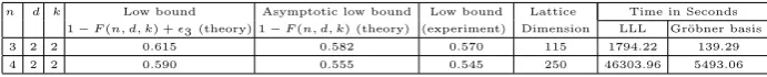
Experimental results.Our results are presented in Table 6. In these experiments, we observe that the condition det(L(n, d, k))< pdk·dimL(n,d,k))is sufficient to find the desired roots. We can easily see that the experiment values are slightly better than the corresponding theoretical results.
Table 6 Experimental results of the third strategy on low bounds of logδ
2p for 1000-bitp.
n d k Low bound Asymptotic low bound Low bound Lattice Time in Seconds 1−F(n, d, k) +3 (theory) 1−F(n, d, k) (theory) (experiment) Dimension LLL Gr¨obner basis
3 2 2 0.615 0.582 0.570 115 1794.22 139.29
4 2 2 0.590 0.555 0.545 250 46303.96 5493.06
Comparison.In order to give the explicit observation on Corollary 3, we present the ratio logδ
2p for small nand differentk in Table 7, where d is optimal for the correspondingn. We can see that the ratio logδ
We give Table 8 and Table 9 to indicate relations between the ratio logδ 2p and
n for optimal d. We have known that the third strategy is same as the second strategy whenk= 1. From Table 8 and Table 9, we can see that the result in the third strategy fork= +∞is more ideal than that in the second strategy.
Compared to the works in [2, 26], we can find that the asymptotic result (k= +∞) of logδ
2p in the third strategy is same as those in [2, 26] for n = 1. The asymptotic results in the third strategy are slightly better than that in [2] but slightly weaker than that in [26] forn= 2 and 3, and logδ
2p <1/2 for n≥4 in the third strategy, which is always better than the results in [2, 26].
Table 7 The ratio logδ
2p about smallnand differentk
P P
PP
k
n 1 2 3 4 5 6
10 0.6818 0.5952 0.5308 0.4980 0.4780 0.4560 d=1 d=2 d=2 d=2 d=2 d=3
20 0.6746 0.5850 0.5230 0.4893 0.4687 0.4492 d=1 d=1 d=2 d=2 d=2 d=3
30 0.6720 0.5806 0.5203 0.4864 0.4654 0.4469 d=1 d=1 d=2 d=2 d=2 d=3
40 0.6707 0.5784 0.5190 0.4849 0.4638 0.4458 d=1 d=1 d=2 d=2 d=2 d=3
50 0.6699 0.5770 0.5182 0.4840 0.4628 0.4451 d=1 d=1 d=2 d=2 d=2 d=3
Table 8 The minimum value of logδ
2pfor fixednin the third strategy
P P
PP
k
n 1 2 3 4 5 6 7 8 9
1 0.7500 0.6667 0.6250 0.5841 0.5611 0.5378 0.5220 0.5073 0.4953
d= 1 d= 2 d= 2,3 d= 3 d= 3 d= 4 d= 4 d= 5 d= 5
+∞ 0.6667 0.5714 0.5085 0.4748 0.4518 0.4369 0.4235 0.4141 0.4066
d= 1 d= 1 d= 2 d= 3 d= 4 d= 3 d= 4 d= 4 d= 5
Table 9 The smallestnneeded for fixed logδ
2pin the third strategy
````
``
k
δ/log2p 0.6678 0.5714 0.5005 0.4953 0.4276 0.3782 0.3419
1 2 3 9 9 20 50 100
+∞ 1 2 4 4 7 16 86
7 Conclusion
For analyzing the modular inversion hidden number problem, we gave a concrete lattice for explaining the best result up to now proposed by Boneh et al., and further improved the lattice construction such that the requirement of samples are fewer. Our attacks on inversive congruential generator improve the existing works.
Acknowledgements.
The authors would like to thank anonymous reviewers for their helpful comments and suggestions.
References
1. Akavia, A.: Advances in Cryptology - CRYPTO 2009: 29th Annual International Cryp-tology Conference, Santa Barbara, CA, USA, August 16-20, 2009. Proceedings, chap. Solving Hidden Number Problem with One Bit Oracle and Advice, pp. 337–354. Springer Berlin Heidelberg, Berlin, Heidelberg (2009). DOI 10.1007/978-3-642-03356-8 20. URL http://dx.doi.org/10.1007/978-3-642-03356-8_20
2. Bauer, A., Vergnaud, D., Zapalowicz, J.C.: Inferring sequences produced by nonlinear pseudorandom number generators using coppersmiths methods. In: M. Fischlin, J. Buch-mann, M. Manulis (eds.) Public Key Cryptography-PKC 2012,Lecture Notes in Com-puter Science, vol. 7293, pp. 609–626. Springer Berlin Heidelberg (2012). DOI 10.1007/ 978-3-642-30057-8 36. URLhttp://dx.doi.org/10.1007/978-3-642-30057-8_36 3. Blackburn, S., Gomez-Perez, D., Gutierrez, J., Shparlinski, I.: Predicting the inversive
generator. In: K. Paterson (ed.) Cryptography and Coding,Lecture Notes in Comput-er Science, vol. 2898, pp. 264–275. Springer Berlin Heidelberg (2003). DOI 10.1007/ 978-3-540-40974-8 21. URLhttp://dx.doi.org/10.1007/978-3-540-40974-8_21 4. Blackburn, S.R., Gomez-perez, D., Gutierrez, J., Shparlinski, I.E.: Predicting nonlinear
pseudorandom number generators. MATH. COMPUTATION74, 2004 (2004)
5. Boneh, D., Halevi, S., Howgrave-Graham, N.: The modular inversion hidden number prob-lem. In: ASIACRYPT 2001, pp. 36–51. Springer (2001)
6. Boneh, D., Venkatesan, R.: Hardness of computing the most significant bits of secret keys in Diffie-Hellman and related schemes. In: CRYPTO 1996, pp. 129–142. Springer (1996) 7. Boyar, J.: Inferring sequences produced by pseudo-random number generators. J. ACM
36(1), 129–141 (1989). DOI 10.1145/58562.59305. URLhttp://doi.acm.org/10.1145/ 58562.59305
8. Comtet, L.: Advanced Combinatorics. D. Reidel Publishing Company (1974)
9. Cox, D.A.: Ideals, varieties, and algorithms: an introduction to computational algebraic geometry and commutative algebra. Springer (2007)
10. Eichenauer, J., Lehn, J.: A non-linear congruential pseudo random number generator. Statistische Hefte27(1), 315–326 (1986). DOI 10.1007/BF02932576. URLhttp://dx. doi.org/10.1007/BF02932576
11. Eichenauer-Herrmann, J., Herrmann, E., Wegenkittl, S.: A survey of quadratic and in-versive congruential pseudorandom numbers, pp. 66–97. Springer New York, New Y-ork, NY (1998). DOI 10.1007/978-1-4612-1690-2 4. URLhttp://dx.doi.org/10.1007/ 978-1-4612-1690-2_4
12. Howgrave-Graham, N.: Finding small roots of univariate modular equations revisited. In: Crytography and Coding, pp. 131–142. Springer (1997)
13. Howgrave-Graham, N.A., Smart, N.P.: Lattice attacks on digital signature schemes. De-signs, Codes and Cryptography23(3), 283–290 (2001). DOI 10.1023/A:1011214926272. URLhttp://dx.doi.org/10.1023/A:1011214926272
14. Lenstra, A.K., Lenstra, H.W., Lov´asz, L.: Factoring polynomials with rational coefficients. Mathematische Annalen261(4), 515–534 (1982)
16. Niederreiter, H.: Random Number Generation and Quasi-Monte Carlo Methods. Society for Industrial and Applied Mathematics (1992). DOI 10.1137/1.9781611970081. URL http://epubs.siam.org/doi/abs/10.1137/1.9781611970081
17. Niederreiter, H.: New developments in uniform pseudorandom number and vector gener-ation. In: H. Niederreiter, P.S. Shiue (eds.) Monte Carlo and Quasi-Monte Carlo Meth-ods in Scientific Computing,Lecture Notes in Statistics, vol. 106, pp. 87–120. Springer New York (1995). DOI 10.1007/978-1-4612-2552-2 5. URLhttp://dx.doi.org/10.1007/ 978-1-4612-2552-2_5
18. Niederreiter, H., Rivat, J.: On the correlation of pseudorandom numbers generated by inversive methods. Monatshefte f¨ur Mathematik153(3), 251–264 (2008). DOI 10.1007/ s00605-007-0503-3. URLhttp://dx.doi.org/10.1007/s00605-007-0503-3
19. Niederreiter, H., Shparlinski, I.: Recent advances in the theory of nonlinear pseudorandom number generators. In: K.T. Fang, H. Niederreiter, F. Hickernell (eds.) Monte Carlo and Quasi-Monte Carlo Methods 2000, pp. 86–102. Springer Berlin Heidelberg (2002). DOI 10.1007/978-3-642-56046-0 6. URLhttp://dx.doi.org/10.1007/978-3-642-56046-0_6 20. Niederreiter, H., Winterhof, A.: On the Structure of Inversive Pseudorandom Number
Generators, pp. 208–216. Springer Berlin Heidelberg, Berlin, Heidelberg (2007). DOI 10. 1007/978-3-540-77224-8 25. URLhttp://dx.doi.org/10.1007/978-3-540-77224-8_25 21. Pirsic, G., Winterhof, A.: On the structure of digital explicit nonlinear and
inver-sive pseudorandom number generators. Journal of Complexity 26(1), 43 – 50 (2010). DOI http://dx.doi.org/10.1016/j.jco.2009.07.001. URLhttp://www.sciencedirect.com/ science/article/pii/S0885064X09000661
22. Shparlinski, I.E.: Playing hide-and-seek with numbers: the hidden number problem, lat-tices, and exponential sums. In: proceeding of symposia in applied mathematics, vol. 62, pp. 153–177 (2005)
23. Stern, J.: Secret linear congruential generators are not cryptographically secure. In: Foun-dations of Computer Science, 1987., 28th Annual Symposium on, pp. 421–426 (1987). DOI 10.1109/SFCS.1987.51
24. Topuzo˘glu, A., Winterhof, A.: On the linear complexity profile of nonlinear congruential pseudorandom number generators of higher orders. Applicable Algebra in Engineering, Communication and Computing16(4), 219–228 (2005). DOI 10.1007/s00200-005-0181-0. URLhttp://dx.doi.org/10.1007/s00200-005-0181-0
25. Winterhof, A.: Recent Results on Recursive Nonlinear Pseudorandom Number Gen-erators, pp. 113–124. Springer Berlin Heidelberg, Berlin, Heidelberg (2010). DOI 10.1007/978-3-642-15874-2 9. URLhttp://dx.doi.org/10.1007/978-3-642-15874-2_9 26. Xu, J., Hu, L., Huang, Z., Peng, L.: Modular inversion hidden number problem revisited.
In: Information Security Practice and Experience, pp. 537–551. Springer (2014)
A The leading monomial of the polynomial in (13)
From (12) and (13), we can deduce
fi0,i1,...,in(x0, x1,· · ·, xn) =x
i0
0 ·(xj1· · ·xjs) +ui0+1,1·h1+· · ·+ui0+1,s·hs.
Since that xi0
0x i1
1 · · ·x in
n is written as xi00 ·(xj1· · ·xjs), thus, our goal is to analyze x
i0
0 ·
(xj1· · ·xjs) is the leading monomial offi0,i1,...,in(x0, x1,· · ·, xn). Note that the polynomial
hl(1≤l≤s) is composed of the terms inglexcept for the corresponding terms of monomials
xj1· · ·xjs, x0·(xj1· · ·xjs),· · ·, x
s−1
0 ·(xj1· · ·xjs). Letxl0
0xk1· · ·xkt be a monomial of ui0+1,1·h1+· · ·+ui0+1,s·hs. Hence, we can obtain
{k1,· · ·, kt} ⊂ {j1, . . . , js}wheret < s. According to the defined order (1), there is
xl0
0 ·(xk1· · ·xkt)≺x
i0
0 ·(xj1· · ·xjs),
which implies that the leading monomial offi0,i1,...,in(x0, x1,· · ·, xn) isx
i0
B Computation of the Determinant ofL(n, d)
Note that the determinant ofL(n, d) is product of the diagonal entries. For the case 1, the contribution ofhi0,i1,···,in(x0, x1,· · ·, xn) to the determinant ofL(n, d) is
d Y
i0=0
pd·Xi0.
For the case 2.a, the contribution ofhi0,i1,···,in(x0, x1,· · ·, xn) to the determinant ofL(n, d) is given by:
d Y
i0=s
d Y
s=1
p(d−s)
n
s
·X(i0+s) n
s
.
For the case 2.b, the contribution offi0,i1,···,in(x0X, x1X,· · ·, xnX) is:
d Y
s=1 s−1 Y
i0=0
p(d+1−s)
n
s
·X(i0+s) n
s
.
To sum up, we get
det(L(n, d)) =pα(n,d)·Xβ(n,d),
whereα(n, d) =d(d+ 1)
d P s=0 n s −d d P s=0
sns
andβ(n, d) =d(d+1)2
d P s=0 n s
+ (d+ 1)
d P s=0
s ns
.
C Computation on pF(n,d)−2
Our goal is to derive a lower bound of
ωω−2n2ω(ω4−1)pdn −β(n,d1 )
·p
dω−α(n,d)
β(n,d) .
First, from the valuesβ(n, d) = d(d+1)2
d P s=0 n s
+ (d+ 1)
d P s=0
s ns
andω= dim(L(n, d)) =
(d+ 1)
d P s=0 n s
, we get β(n,d)ω < d+22 . Further, there is
ωω−2n2ω(ω4−1)pdn β(n,d1 )
< ωd+21 2
ω−1 2(d+2)p
dn
β(n,d) =p2,
where2=2 log2ω+ω−1
2(d+2) log2p +
dn β(n,d).
Second, plugging the valuesω,α(n, d) andβ(n, d) intodωβ(n,d)−α(n,d), we get that
dω−α(n, d)
β(n, d) =
2d d P s=0
sns
d(d+ 1)
d P s=0 n s
+ 2(d+ 1)
d P s=0
sns
=F(n, d).
Thus,
ωω−2n2ω(ω4−1)pdn
− 1
β(n,d)
·p
dω−α(n,d)
D Analysis of the polynomial in (19)
First, we analyze the leading monomial of the polynomial. We know that the leading monomial of the polynomial in (19) is the product of the leading monomials of the following polynomials:
g(xs1
0 ;S1),· · ·, g(x sl
0 ;Sl), g(x
i0−(s1+···+sl)
0 ;Sl+1), g(x 0
0;Sl+2),· · ·, g(x00;Sm).
Note that the leading monomials ofg(xs1
0 ;S1),· · ·, g(x sl
0;Sl) are respectively xs1·(xj
1· · ·xjs1),· · ·, x
sl·(xj
1· · ·xjsl), the leading monomial of g(xi0−(s1+···+sl)
0 ;Sl+1) is xi0
−(s1+···+sl)·(xj1· · ·xjsl
+1) and the
leading monomials ofg(x00;Sl+2),· · ·, g(x00;Sm) are respectively
(xj1· · ·xjsl+2),· · ·,(xj1· · ·xjsm).
It is easy to compute that the leading monomial of the polynomial in (19) is
xi0·(xj
1· · ·xjs1)·(xj1· · ·xjs2)· · ·(xj1· · ·xjsm) which is equal toxi0
0 x i1
1 · · ·x in
n from (18) directly. Hence, the leading monomial of the
poly-nomial in (19) isxi0
0 x i1
1 · · ·x in
n.
Next, we show that the polynomial in (19) has the following relation
fi0,i1,...,in(x0, x1,· · ·, xn) = 0 modp
(i1+···+in)−(m−l).
Note that the polynomials in (19) are composed of the polynomials generated by the second strategy. From|S1|=s1,· · ·,|Sl|=sl, we have
g(xs1
0 ;S1) = 0 modp
s1,· · ·, g(xsl
0 ;Sl) modp sl.
Froms1+· · ·+sl≤i0<(s1+· · ·+sl) +sl+1, we get 0≤i0−(s1+· · ·+sl)< sl+1=|Sl+1|,
thus there is
g(xi0−(s1+···+sl)
0 ;Sl+1) = 0 modp
sl+1−1.
According to|Sm| ≥ · · · ≥ |Sl+2| ≥ |Sl+1|=sl+1>0, we obtain
g(x00;Sl+2) = 0 modpsl+2
−1,· · ·, g(x0
0;Sm) = 0 modpsm
−1.
Therefore, we getfi0,i1,...,in(x0, x1,· · ·, xn) = 0 modp(s1+
···+sm)+(m−l).From (18), we have s1+· · ·+sm=i1+· · ·+in. Hence
fi0,i1,...,in(x0, x1,· · ·, xn) = 0 modp
(i1+···+in)−(m−l).
E Computation on Dimension and Determinant ofL(n, d, k)
Let
S(n, d, k) ={(i1,· · ·, in),0≤i1,· · ·, in≤k,0≤i1+· · ·+in≤dk}.
Denote|S(n, d, k)|is the cardinality ofS(n, d, k). Note that|S(n, d, k)|can also be regarded as the sum of coefficients of thexs in the expansion of the polynomial (1 +x+· · ·+xk)n, s= 0,1,· · ·, dk. Namely,|S(n, d, k)|=
dk P s=0
n s
k+1.
First, we compute the dimension ofL(n, d, k). Clearly, the dimension of the latticeL(n, d, k) is equal to the number of vectors inI(n, d, k), which can be expressed as (dk+ 1)· |S(n, d, k)|, Therefore,
dim(L(n, d, k)) = (dk+ 1)
dk X
s=0
n
s
Then, we compute the determinant ofL(n, d, k). Since that the determinant ofL(n, d, k) is product of the diagonal entries where all tuples (i0, i1,· · ·, in)∈I(n, d, k), we consider the following cases.
For the case 1 and case 2.a, the contribution ofhi0,i1,···,in(x0, x1,· · ·, xn) to the deter-minant ofL(n, d) is
Y
(i1,···,in)∈S(n,d,k) dk Y
i0=i1+···+in
pdk−(i1+···+in)·Xi0+i1+···+in,
wherei1+· · ·+in= 0 in the case 1 andi1+· · ·+in>0 in the case 2.a.
For the case 2.b, the contribution ofhi0,i1,···,in(x0X, x1X,· · ·, xnX) is given as follows:
Q (i1,···,in)∈S(n,d,k)
m−1 Q l=0
s1+s2+···+sl+1−1
Q i0=s1+s2+···+sl
pdk−(i1+···+in)+(m−l)·Xi0+i1+···+in ,
which can be rearranged as
Y
(i1,···,in)∈S(n,d,k)
p
m−1 P
l=0
(m−l)sl+1
·
i1+···+in−1 Y
i0=0
pdk−(i1+···+in)·Xi0+i1+···+in
according to the relations1+· · ·+sm=i1+· · ·+inin (18). Thus, we can get that det(L(n, d, k)) =
Y
(i1,···,in)∈S(n,d,k)
p
m−1 P
l=0
(m−l)sl+1
· dk Y
i0=0
pdk−(i1+···+in)·Xi0+i1+···+in
.
First, let us compute Q (i1,···,in)∈S(n,d,k)
dk Q i0=0
pdk−(i1+···+in).We can deduce that
X
(i1,···,in)∈S(n,d,k) dk X
i0=0
(dk−(i1+· · ·+in))
=dk(dk+ 1)· P (i1,···,in)∈S(n,d,k)
1−(dk+ 1)· P (i1,···,in)∈S(n,d,k)
(i1+· · ·+in)
=dk(dk+ 1)
dk P s=0 n s
k+1−(dk+ 1) dk P s=0
s ns k+1
wheres=i1+· · ·+in. Hence,
Y
(i1,···,in)∈S(n,d,k)
dk Y
i0=0
pdk−(i1+···+in)=p
dk(dk+1)dkP
s=0 n
s
k+1−(dk+1)
dk
P
s=0
sns
k+1.
Second, let us compute Q
(i1,···,in)∈S(n,d,k) dk Q i0=0
Xi0+i1+···+in.Note that
X
(i1,···,in)∈S(n,d,k)
dk X
i0=0
(i0+i1+· · ·+in)
=dk(dk+1)2 · P (i1,···,in)∈S(n,d,k)
1−(dk+ 1)· P (i1,···,in)∈S(n,d,k)
(i1+· · ·+in)
=dk(dk+1)2
dk P s=0 n s
k+1−(dk+ 1) dk P s=0
Therefore,
Y
(i1,···,in)∈S(n,d,k)
dk Y
i0=0
Xi0+i1+···+in=X dk(dk+1)
2 dk P s=0 n s
k+1−(dk+1)
dk
P
s=0
sns
k+1.
Third, let us compute Q
(i1,···,in)∈S(n,d,k)
p
m−1 P
l=0
(m−l)sl+1
. We can rewrite
m−1 P l=0
(m−l)sl+1=
m−1 P l=0
(sl+1−sl)(1 +· · ·+m−l)
wheres0= 0. Note that there are exactly (sl+1−sl) entries that are equal to (m−l) in the exponent set{i1,· · ·, in}forl= 0,1,· · ·, m−1. Hence,
m−1 P l=0
(sl+1−sl)(1 +· · ·+m−l) can be regarded as a rearrangement of (1 +· · ·+i1) +· · ·+ (1 +· · ·+in), which is computed as
i1+···+in+i21+···+i2n
2 . Therefore,
X
(i1,···,in)∈S(n,d,k)
m−1 X
l=0
(t−l)sl+1= X
(i1,···,in)∈S(n,d,k)
i1+· · ·+in+i2
1+· · ·+i2n
2 .
We have known P
(i1,···,in)∈S(n,d,k)
(i1+· · ·+in) =
dk P s=0
sns
k+1.Next, we analyze
X
(i1,···,in)∈S(n,d,k)
i21+· · ·+i2n
.
Since
X
(i1,···,in)∈S(n,d,k)
i21+· · ·+i2n
=n· X
(i1,···,in)∈S(n,d,k) i2n
Here, 0≤in≤kand 0≤(i1+· · ·+in−1)≤min{dk−in,(n−1)k}as (i1,· · ·, in)∈S(n, d, k).
Thus, we can rewrite the above relation using polynomial coefficients:
X
(i1,···,in)∈S(n,d,k)
i21+· · ·+i2n
=n· k X
i=0
min{dk−i,(n−1)k}
X
s=0 i2
n−1 s
k+1 .
Further, we obtain
Y
(i1,···,in)∈S(n,d,k)
p
m−1 P
l=0
(m−l)sl+1
=p n 2· k P i=0
min{dk−i,(n−1)k} P
s=0
i2n−s1
k+1+ 1 2
dk
P
s=0
sns
k+1.
According to the above analysis, we get det(n, d, k) =pα(n,d,k)·Xβ(n,d,k), whereα(n, d, k)=
dk(dk+ 1)
dk X s=0 n s k+1 +n 2 k X i=0
min{dk−i,(n−1)k}
X
s=0 i2
n−1 s
k+1
−2dk+ 1
2 dk X s=0 s n s k+1 and
β(n, d, k) =dk(dk+ 1) 2 dk X s=0 n s k+1
+ (dk+ 1)
F Computation onpF(n,d,k)−3
Our goal is to show a lower bound of
ωω−2n2ω(ω4−1)pndk
− 1
β(n,d,k)
·p
dkω−α(n,d,k)
β(n,d,k)
whereω= dim(L(n, d, k)).
First, from the values dim(L(n, d, k)) andβ(n, d, k), we get β(n,d,k)ω <dk+22 , furthermore,
ωω−2n2ω(ω4−1)pndk
β(n,d,k1 )
< ωdk1+22
ω−1 2(dk+2)p
ndk β(n,d,k) =p3
where3=2 log2ω+(ω−1)
2(dk+2) log2p + ndk β(n,d,k).
Second, according to the valuesα(n, d, k),β(n, d, k),ωandF(n, d, k), we can compute
dkω−α(n, d, k)
β(n, d, k) =F(n, d, k). Therefore, there is the following relation
ωω−2n2ω(ω4−1)pndk
− 1
β(n,d,k)
·p
dω−α(n,d,k)
β(n,d,k) > pF(n,d,k)−3.
G Sage Code for the first strategy
n=14
P=ZZ.random_element(2^999,2^1000) P=next_prime(P)
a=ZZ.random_element(P) X=[]
B=[] E=[] bb=1000-536
for i in range(n+1): xi=ZZ.random_element(P) X.append(xi)
yi=(a+xi).inverse_mod(P) bi=yi-yi%2^bb
ei=yi%2^bb B.append(bi) E.append(ei)
R.<z0,z1,z2,z3,z4,z5,z6,z7,z8,z9,z10,z11,z12,z13,z14>=QQ[] Z=[z0,z1,z2,z3,z4,z5,z6,z7,z8,z9,z10,z11,z12,z13,z14] # U is the upper bound of the root
U=ZZ.random_element(2^(bb-1),2^(bb)) G=[]
H=[]
for i in range(n+1): for j in range(i+1,n+1):
Aij=X[i]-X[j]
Bij=X[i]*B[j]-X[j]*B[j]+1 Cij=X[i]*B[i]-X[j]*B[i]-1
f=Aij*Z[i]*Z[j]+Bij*Z[i]+Cij*Z[j]+Dij bn=(Aij).inverse_mod(P)
g=Z[i]*Z[j]+(Bij*bn)%P*Z[i]+(Cij*bn)%P*Z[j]+(Dij*bn)%P G.append(g)
H=union(H,g.monomials())
for i in range(n+1): G.append(Z[i]*P) G.append(1*P)
cc=Set(H).cardinality()
print ’Dimension of the Lattice=’, cc M=matrix(ZZ,cc,cc,range(cc*cc)) for i in range(cc):
g=R(G[i])(z0*U,z1*U,z2*U,z3*U,z4*U,z5*U,z6*U,z7*U,z8*U,z9*U,z10*U,z11*U,z12*U,z13*U,z14*U) for j in range(cc):
cij=g.coefficient(H[j])(0,0,0,0,0,0,0,0,0,0,0,0,0,0,0) M[i,j]=cij
tt=cputime() M=M.LLL()
print ’Time of LLL algorithm’,cputime(tt) F=[]
M3=[]
for j in range(116): f1=0
for i in range(cc):
f1=f1+(M[j][i]/H[i](U,U,U,U,U,U,U,U,U,U,U,U,U,U,U))*H[i]
M3.append(f1)
I=(M3)*R tt=cputime()
B=I.groebner_basis()
print ’Time of Groebner basis’, cputime(tt) print B[0],E[0]
H Sage Code for the second strategy
P=ZZ.random_element(2^999,2^1000) P=next_prime(P)
n=4 d=3
a=ZZ.random_element(P) X=[]
B=[] E=[] bb=1000-555
for i in range(n+1): xi=ZZ.random_element(P) X.append(xi)
ei=yi%2^bb B.append(bi)
E.append(ei)
R.<z0,z1,z2,z3,z4>=QQ[] Z=[z0,z1,z2,z3,z4]
G=[] H=[] a=0 G2=[] i=0
for j in range(1,n+1): Aij=X[0]-X[j]
Bij=X[0]*B[j]-X[j]*B[j]+1 Cij=X[0]*B[0]-X[j]*B[0]-1
Dij=(X[0]-X[j])*B[0]*B[j]+B[0]-B[j] f=Aij*Z[0]*Z[j]+Bij*Z[0]+Cij*Z[j]+Dij bn=(Aij).inverse_mod(P)
g=Z[0]*Z[j]+(Bij*bn)%P*Z[0]+(Cij*bn)%P*Z[j]+(Dij*bn)%P G.append(g)
G2.append([i,j]) H=union(H,g.monomials())
# U is the upper bound of the root U=ZZ.random_element(2^(bb-1), 2^bb)
f=0
for i1 in range(n):
for i2 in range(i1+1,n): for i3 in range(i2+1,n):
f=f+G[i1]*G[i2]*G[i3]
M=(f).monomials() ll=len(M)
print ’Dimension of the Lattice=’, ll
F=[]
for i in range(len(M)): ss=M[i]
s0=diff(M[i],z0)(1,1,1,1,1) s1=diff(M[i],z1)(1,1,1,1,1) s2=diff(M[i],z2)(1,1,1,1,1) s3=diff(M[i],z3)(1,1,1,1,1) s4=diff(M[i],z4)(1,1,1,1,1)
else:
s=s1+s2+s3+s4 if(s0>=s):
f=z0^(s0-s)*(G[0])^s1*(G[1])^s2*(G[2])^s3*(G[3])^s4 F.append(f*P^(d-s))
else: F2=[] F3=[] F4=[] if(s1==1):
F2.append(z1) F3.append(G[0])
if(s2==1): F2.append(z2) F3.append(G[1])
if(s3==1): F2.append(z3) F3.append(G[2])
if(s4==1): F2.append(z4) F3.append(G[3])
for i in range(len(F2)): f=1
for j in range(len(F2)): if(j==i):
f=f*F2[i]
else: f=f*F3[j]
F4.append(f)
F1=[]
for j in range(s):
F1.append(z0^j*z1^s1*z2^s2*z3^s3*z4^s4) if(s>1):
R1=IntegerModRing(P^(s-1)) MS=Matrix(R1,s,s,range(s*s))
for j in range(s): for l in range(s):
MS[j,l]=0
for j in range(s): for l in range(s):
cjl=(F4[j]).coefficient(F1[l]) cjl=cjl(0,0,0,0,0)
MS[j,l]=cjl
MSIN=MS.inverse()
F5=[]
for j in range(s):
f=f+ZZ(MSIN[l][j])*F4[j] S2=f.monomials()
g=0
for j in range(len(S2)): cj=f.coefficient(S2[j]) cj=cj(0,0,0,0,0) cj=cj%P^(s-1) cj=ZZ(cj) g=g+cj*S2[j] f=g
F.append(f*P^(d+1-s)) else:
F.append(F4[j]*P^d)
rr=len(F)
M2=Matrix(ZZ,rr,rr,range(rr*rr)) for i in range(rr):
f=F[i]
f=f(z0*U,z1*U,z2*U,z3*U,z4*U) for j in range(len(M)):
cij=f.coefficient(M[j]) cij=cij(0,0,0,0,0) M2[i,j]=cij tt=cputime() M2=M2.LLL()
print ’LLL Time’,cputime(tt) M3=[]
for j in range(25): f1=0
for i in range(rr):
f1=f1+(M2[j][i]/M[i](U,U,U,U,U))*M[i] M3.append(f1)
I=(M3)*R tt=cputime()
B=I.groebner_basis()
print ’Groebner Basis Time’, cputime(tt) print B[0],E[0]
I Sage Code for the third strategy
P=ZZ.random_element(2^999,2^1000) P=next_prime(P)
n=3 d=2 k=2
a=ZZ.random_element(P) X=[]
B=[] E=[] bb=1000-570
for i in range(n+1): xi=ZZ.random_element(P) X.append(xi)
bi=yi-yi%2^bb ei=yi%2^bb B.append(bi)
E.append(ei)
R.<z0,z1,z2,z3>=QQ[] Z=[z0,z1,z2,z3] G=[]
H=[]
G2=[]
for j in range(1,n+1): Aij=X[0]-X[j]
Bij=X[0]*B[j]-X[j]*B[j]+1 Cij=X[0]*B[0]-X[j]*B[0]-1
Dij=(X[0]-X[j])*B[0]*B[j]+B[0]-B[j] f=Aij*Z[0]*Z[j]+Bij*Z[0]+Cij*Z[j]+Dij bn=(Aij).inverse_mod(P)
g=Z[0]*Z[j]+(Bij*bn)%P*Z[0]+(Cij*bn)%P*Z[j]+(Dij*bn)%P print g(E[0],E[1],E[2],E[3])%P
G.append(g) G2.append([i,j]) H=union(H,g.monomials())
#U is the upper bound of the root U=ZZ.random_element(2^(bb-1), 2^bb)
#This is the starting position for polynomial generation for Case 2.b of the paper
M=[]
for i0 in range(n): for i1 in range(1+1):
for i2 in range(1+1): for i3 in range(1+1):
if(i1+i2+i3<=n):
M.append(z0^i0*z1^i1*z2^i2*z3^i3)
F33=[] F44=[]
for i in range(len(M)): ss=M[i]
s0=diff(M[i],z0)(1,1,1,1) s1=diff(M[i],z1)(1,1,1,1) s2=diff(M[i],z2)(1,1,1,1) s3=diff(M[i],z3)(1,1,1,1)
if(s1+s2+s3==0): F33.append(M[i]) F44.append(0)
s=s1+s2+s3 if(s0>=s):
f=z0^(s0-s)*(G[0])^s1*(G[1])^s2*(G[2])^s3 F33.append(f)
F44.append(s)
else: F2=[] F3=[] F4=[] if(s1==1):
F2.append(z1) F3.append(G[0])
if(s2==1): F2.append(z2) F3.append(G[1])
if(s3==1): F2.append(z3) F3.append(G[2])
for i in range(len(F2)): f=1
for j in range(len(F2)): if(j==i):
f=f*F2[i]
else: f=f*F3[j]
F4.append(f)
F1=[]
for j in range(s):
F1.append(z0^j*z1^s1*z2^s2*z3^s3)
if(s>1):
R1=IntegerModRing(P^(s-1)) MS=Matrix(R1,s,s,range(s*s))
for j in range(s): for l in range(s):
MS[j,l]=0
for j in range(s): for l in range(s):
cjl=(F4[j]).coefficient(F1[l]) cjl=cjl(0,0,0,0)
MS[j,l]=cjl
MSIN=MS.inverse()
F5=[]
for l in range(s0,s0+1): f=0
for j in range(s):