The role of mutation in the optimisation of numeric functions by genetic algorithms

VICTORIA

!

UNIVERSITY

-

·

.· 0

~

~ . . 0

..

·. ~

DEPARTMENT OF COMPUTER AND

MATHEMATICAL SCIENCES

The Role of Mutation in the Optimisation of

Numeric Functions by Genetic Algorithms

Robert Hinterding, Harry Gielewski and

Tom C

. Peachey

(68 CO:MP 22)

February, 1996

(AMS

: 68T05)

TECHNICAL REPORT

VICTORIA UNIVERSITY OF TECHNOLOGY

DEPARTMENT OF CO:MPUTER AND MATHEMATICAL SCIENCES

P 0

BOX 14428

MCMC

MELBOURNE, VICTORIA 8001

AUSTRALIA

DEPARTMENT OF COMPUTER AND

MATHEMATICAL SCIENCES

The Role of Mutation in the Optimisation of

Numeric Functions by Genetic Algorithms

Robert Hinterding

email: [email protected]

Harry Gielewski

email:[email protected]

T. C

.

Peachey

email: [email protected]

TECHNICAL REPORT

68COMP22

December 1995

Department of Computer and Mathematical Sciences

VICTORIA UNIVERSITY OF TECHNOLOGY

PO Box 14428 MMC, Melbourne 3000, Australia

Abstract

Normally in Genetic Algorithms, mutation is considered a background operator and the genes are considered to be the binary bits of the chromo-some. In this paper we take a different viewpoint. We treat the variables of numerical functions as the genes, and consider the mutation of these genes. We also investigate the role of mutation as an independent repro-duction operator. Our results show the value of this view, and explain some previous comparisons with Evolutionary Strategies.

1

Introduction

In this paper we look at the nature of mutation in Genetic Algorithms ( GAs) used in optimisation of numerical functions. Current theory of GAs considers that mutation is a background operator and just used to provide bits lost by crossover (Holland, 1992). This relies on the view that the genes in a chromo-some are binary bits, and is supported via the current schema theory (Holland, 1992; Goldberg, 1989). Further, current guidelines recommend using genes with

a small alphabet so that the largest number of schema will exist. We however,

find it is useful to view each complete variable in the objective function as a gene.

Gray coding is frequently used in numerical optimisation GAs; the use is justified by the fact that in Gray code, successive numbers differ in only one bit. But is not understood why Gray coding is more effective than binary representation for some functions and not for others.

Hoffmeister and Back (1992) compared GAs to Evolutionary Strategies(ESs) for a number of functions. However the GA parameter settings differed signif-icantly from the standard ones in that all variables were represented using 32 bits. The reason these authors gave was to maintain the same resolution for the object variables as is used in ESs. We investigate the effect of the number of bits in the variable representation on the performance of GAs.

2

Background

Genetic Algorithms ( GAs) and Evolutionary Strategies (ESs) are the main areas of Evolutionary Computation that are used for numerical function optimisation. GAs were introduced in the USA by Holland (1992) in the framework of adap-tation in artificial systems. They are characterised by using a binary encoding,

viewing crossover as the major reproduction operator, with mutation seen as a "background" operator used to replace allele values lost by crossover and se-lection. ESs were introduced in Germany by Rechenberg (1973) and were first applied to experimental optimisation problems with continuous parameters.

Some of the differences between GAs and ESs are: the role of mutation; the representation of variables; and whether mutation works on the genotype or the phenotype. The issues we address in relation to GAs are those of representation and the role and function of mutation. In GAs, genes are normally considered to be the binary bits of the chromosome. We will consider the complete variables of the objective function as the genes and then look at the effect of bit flip mutation on these genes. We will investigate the role and function of mutation in GAs by considering it to be an independent reproduction operator.

3

Representation of Genes and Mutation

It is well known both in GA theory and in natural evolutionary theory that without mutation, evolution would stagnate. That is, once combinations of variants in the current population have explored, no new variations are possible. There is argument about what the unit of evolution is (Dawkins, 1982), but genes are considered to be the best bet. There is no rigid definition of what a gene is, it can be hundreds of nucleotides long, and the definition is really a functional one. That is, it should have a consistent phenotypic effect, although this effect is not completely independent of the other genes on the chromosome. When we consider genes as bits, there is very little consistency between the genotypic and phenotypic values. The effect of the gene is determined by the function variable it maps to and then its position within the gene. We argue this effect is more like that of a nucleotide within a gene, than a gene within a chromosome. When we consider the function variables as a genes, the phenotypic effect is then determined by the function variable it maps to. Further, mutation can now be viewed as a change to the function variable, and its effects can be quantified. ·

3.1

Function Variables as Genes

By treating the function variables as genes, a GA can be more easily seen as searching for values of the function variables (genes) that will produce the optimum.

There are several consequences of this view:

• The number of genes in a numeric GA is now the number of variables in the objective function (see Fig 1). This is now much smaller.

·• The size of the alphabet of a gene is 2n, where n is the length of the gene in bits. This is much larger than before.

• We can now explore the effects of mutation on a gene. Before we could only flip a bit.

Traditional GA:

2 variables, each 4 bits; 8 genes

I

gl

I

gl

I

gl

I

gl

I

g2

I

g2

I

g2

I

g2

I

Variables as genes:

2 variables, each 4 bits; 2 genes

Figure 1: Gene Representation

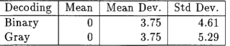
Table 1: Mutation statistics

Decoding Mean Mean Dev. Std Dev.

Binary 0 3.75 4.61

Gray 0 3.75 5.29

demonstrated that where large alphabet sizes are used for genes, the GAs still have very good performance.

Another class of GAs which use function variables as genes are real coded GAs (Davis, 1985; Wright, 1991) as are most ESs. Our approach is different as

we still use bit-flip mutation while viewing the function variables as genes.

3.2 Effect of bit-flip mutation on a Gene

We consider the changes in the value of a gene when one of the bits in the binary string representing that gene is flipped. Select one of the bits in the string, with all bits equally likely, and reverse the polarity of that bit. Both the original string and the new one are decoded and the change calculated. We are concerned with the probability distribution of these changes and how it is affected by the type of representation used.

For the case of 4 bit strings, Table 1 compares statistics of the distribution for Gray decoding with that for fixed point decoding. As expected, the two

representations give a mean of zero. They show identical mean deviations, but

Gray code gives a larger standard deviation.

The probability distributions of changes are shown in Figure 2. With bi-nary coding the allowed changes all have the same probability, but the interval between these values increases exponentially. With Gray code all odd values

0.25 0.2 Prob. O.l 5

0.1 0.05

0

Probability Distributions

I I I I

.... _{binary en< ioding -}

-....

--

--

-I I II I

Probability Distributions 0 .25

....---..--~~----0.2 Prob. 0.15 0.1 0.05

Gray e m g

-0 LL..L.J...U.U....L.L...L..UJ....L..L..J...JJ.LJ....L.L..l.IL.J...JU...W..J...J...WJ

-15 -10 -5 0 5 10 15

Change in gene value -15 -10 -5 Change in gene value 0 5 10 15 Figure 2: Prob. dist for binary and Gray encodings

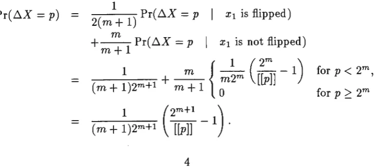
3.2.1 The General Case

Now we consider the general case of a string of length n. We write the string as

X1 x2 .•• Xn and the value represented as x. The change in x caused by changing

one bit will be a random variable ~X. We need to consider only positive changes since the distributions are clearly symmetric.

For binary coding, changing the kth bit from 0 to 1 increases the value by 2n-k. So the distribution is

1

Pr(~X = p) =

2n for p = 2n-k, k = 1,2, . .. n. For the case of Gray coding, the probability distribution is

1 ( 2n )

Pr(~X =

p)

= n ₂n

[[p]) -

1 for p = 1, 3, 5, ... , 2n - 1,

where we use

[[p]]

to denote the largest power of 2 not exceeding positive p.

This result is most easily proved by induction. It is clearly true for n = 1. Suppose it to be true for n = m; we consider the case n = m

+

1. If the binary strings x1x 2 ... Xm+1 are in order of the numbers represented, then the first 2m

have x₁

=

0 while the rest of the strings cycles through a Gray code on m bits. The remaining strings have x1 = 1 and the rest of the strings again cycle through

the Gray code, but in reverse order. So the changes in the values represented, caused by flipping xi, may take the values ±1, ±3, ±5, ... , ±(2m+l - 1), all

being equally likely. On the other hand, if x1 is unchanged then the changes

follow the probability distribution for the case n = m. Thus, considering only

the cases where p is positive,

Pr(~X

=

p)

( 1 ) Pr( ~X

=

p x1 is flipped)

2m+1

m

+

Pr( ~X = p

I

x1 is not flipped)

m+l

( m

+

~

)2m+l

+

m:

1 {

';~m

(

[~]

-1

)

for p

<

2m,

(m

+

~)2m+l (2[~~]

1

This completes the induction on n.

The proof however, obscures the relationship with the distribution for fixed point code. If the kth bit of the n bit string is the one flipped, then for fixed point coding, the change in the decoded value is ±2n-k and there are 2n-I different numbers that may suffer each change. With Gray coding, changing the kth bit causes changes in the values with absolute size 1, 3, 5, ... , 2n-k+I - 1 and there are 2k-I numbers that may undergo each change. It follows that the mean change is the same in each case. The second distribution can be obtained from the first by taking each probability peak and spreading it symmetrically. So the second distribution will have the same mean deviation and a greater standard deviation.

3.2.2 Limiting Distributions

We now consider the effect increasing n on the distribution of changes for the Gray coding case. Clearly, as n - oo, each Pr{ AX = p} - 0 while the total probabality is maintained at 1 by the creation of more possible values of p. A more relevant treatment supposes that all binary strings represent a variable, say

z,

in a fixed range; for convenience we assume

[O, 1).

Then increasing the string length produces a finer granularity in the representation. The question is how the choice of n effects the probability density. Is there a continuous distribution that can be used to represent the limiting case n - oo in the same way that a normal distribution is used as the limiting case of a binomial?

We write AZ for the random variable representing the changes in z and Az for the values that it can take. Note that for a string of length n, the changes caused by a flipping a single bit may take only the dyadic values Az = ±p/2n where pis an odd integer in the range 1 to 2n -1. A particular value Az = p/2r may only occur when the string length n = r. For greater n the closest occuring changes are p/2r

±

1/2n. So we take the probability density at p/2r to be

2 n-I [ Pr{AZ = -p + -1 } + Pr{AZ = -p - -1 }]

2r 2n 2r 2n

2n-I [Pr{ AX= p2n-r + 1} +Pr{ AX= p2n-r - 1}]

1 { 2n 2n }

2n

[[p

2n-r

+

1}}

+

[[p

2n-r _

1}} -

2

·

Since the terms inside the braces are independent of n

>

r this expression approaches 0. The one exception is for Az = 0 when the probability density is (2n -

1)/n

and this -

oo

as n -

oo.

So the probability density distribution becomes more and more concentrated near Az = 0 as n increases. The limiting distribution exists only in the generalized sense of a Dirac delta located at the ongm.

3.3

Granularity of representation

In the previous section we considered the binary strings to represent integers in the range 0 to 2n - 1. In numerical optimisation, the strings more typically represent fractions of the form p/2n where p is an integer. The choice of the number of bits per gene n, controls the spacing between adjacent values, known as the "granularity" of the representation.

We show that, as n is increased, the probability distributions of the changes becomes more and more concentrated about zero. The practical significance of this is that for fine granularity, most mutation steps will be very small. If

the utility of mutation is to directly advance toward the optimum, rather than just supply variation for crossover to work on, then fine granularity will slow convergence.

The other effect of decreasing the granularity is to enlarge the search space.

4

N urneric GA Test functions

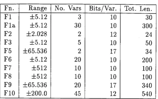
The test functions have· been taken from a number of sources, and more difficult functions have been included. Fl - F5 are from De Jong (1975), F6 - F8 are from Gordon

&

Whitley (1993), F9 is from Hoffmeister and Back (1992), and FlO is from Michalewicz (1994). The range, number of variables and number of bits used to represent each variable is summarised in Table 2.

• Fl Sphere Model. This is a continuous, strictly convex, unimodal func-tion. The solution is at

x*

=

(0, ... , o)T;

fi(x*)

=

0. This is a scalable problem, with n = 3 the problem is easy, Hoffmeister

&

Back (1992) use

n = 30, which we call test function Fla.

• F2 Rosenbrock's Function. This is a continuous, unimodal, bi-quadratic function of two variables. It is a standard test function in optimisa-tion which was proposed by Rosenbrock (1960). The soluoptimisa-tion is at

x*

= (1, l)T;

fi(x*)

=

0.

• F3 De Jong Step Function. This is a simple linear but discontinuous func-tion, which consists of many small plateaus. Due to this characteristic f3 has a lot oflocal optima. The solution is at Xi E [-5.12, ... , -5);

h(

x*)

=

0.

• F5, Shekel's Foxholes. This is a continuous, non-linear, multimodal func-tion proposed by Shekel (1971). It is a difficult problem as it consists of a large plateau with some holes in it which have different objective values at their bottoms, while the plateau is made up of equal objective values. The solution is at

xi=

(-32, -32f;

fs(x*)

~ 1.

Table 2: Function Characteristics

Fn. Range No. Vars Bits/Var. Tot. Len.

Fl ±5.12 3 10 30

Fla ±5.12 30 10 300

F2 ±2.028 2 12 24

F3 ±5.12 5 10 50

F5 ±65.536 2 17 34

F6 ±5.12 20 10 200

F7 ±512 10 10 100

F8 ±512 10 10 100

F9 ±65.536 20 17 340

FlO ±200.0 45 12 540

(1990) as a test function for distributed parallel ESs. The solution is at

x* = (0, ... , O)T; f6(x*) = 0.

• F7, Schwefel's Function. This is a multimodal function characterised by a second-best minimum which is far away from the global optimum. The solution is at x* = (421, ... ,42l)T; h(x*) = 0.

• F8, Griewangk's Function. This function is difficult for GAs because the product term causes the 10 variables to be strongly independent. The solution is at x* = (0, . .. ,o)T;f8(x*) = 0.

• F9, Schwefel's Problem 1.2. This is a continuous, unimodal function which comes from the set of test functions that Schwefel (1977) once used to compare the performance of several optimisation methods. The difficulty of this function results from the fact that searching along the coordinate axes only gives a poor rate of convergence. The solution is at x* =

(0, .. . ,o)T;fg(x*)

=

o.

• FlO, Michalewicz's dynamic control problem. The range of x is (-200, 200), the function has a minimum at 16,180.4.

5

The GA

The Genetic Algorithm used is a steady-state GA based on the description of OOGA in Davis (1991). Tournament selection is used with a tournament size of 2 as this was faster and gave comparable results to roulette wheel selection with linear normalisation. It was developed using Smalltalk/V for Windows. The following parameters can be set:

• Allow Duplicates - set a flag to allow or disallow duplicates to exist in the population. If duplicates are not allowed, any duplicates produced by reproduction are discarded while they still count as an evaluation. We determine whether two chromosomes are the same by comparing their genotypes.

• Number of Evaluations - set the number of evaluations for the run. We use evaluations rather than generations so that we can compare between runs where the population size and replacement rate are different.

• Replacement Rate - set the percentage of the population that will be replaced by reproduction in one generation. The rate can be set from O to 1003.

• Crossover Rate - set the percentage of the replacement population that will be replaced by crossover in one generation. The remainder of the replacement population will be produced by mutation. The rate can be set from 0 to 100%.

• Poisson Mutation - use a Poisson distributed random variable to deter-mine how many genes to mutate in a chromosome.

• Poisson Mean - set the mean (

.X)

for the Poisson distributed random variable.

Two point crossover was used for all the experiments, although others were available.

In the Genetic Algorithm used, a new chromosome is produced either by crossover or mutation but not both. In this way we treat crossover and mutation as independent reproduction operators. This was done so that the separate effects of these reproduction operators could be determined. By using these operators independently and varying the application rates we can determine the mix of these operators that produces the best results within a given number of evaluations.

The mutation rate for the GA is (100% - Crossover rate). The mutation rate is the percentage of chromosomes of the replacement population that will undergo mutation. If Poisson Mutation is false, then mutation of one gene is carried out. If Poisson Mutation is true, then the number of genes to be mutated in a chromosome is determined by sampling a Poisson distributed random variable with mean 1. If n genes are to be mutated in a chromosome, then we repeat n times: select a random gene from the chromosome and flip a randomly selected bit in the gene.

6

The Experiments

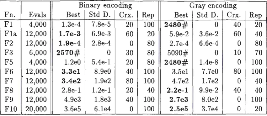
Table 3: Results from Set 1 and 2 runs

Binary encoding Gray encoding

Fn. Evals Best Std D. Crx. Rep Best Std D. Crx. Rep Fl 4,000 l.3e-4 7.8e-5 20 100 2480# 0 40 20 Fla 12,000 1. 7e-3 6.9e-3 60 20 5.9e-2 3.6e-2 60 40 F2 12,000 1.9e-4 2.8e-4 0 80 2.7e-4 6.6e-4 0 80

F3 6,000 2570# 0 30 80 5090# 0 10 70

F5 4,000 l.2e0 5.4e-l 20 80 2480# l.4e-8 0 100 F6 12,000 3.3el 8.9e0 40 100 3.5el 7.7e0 80 100 F7 12,000 3.4e2 l.9e2 80 100 4.7e2 l.7e2 0 40 F8 12,000 2.8e-l l.2e-l 20 40 2.2e-1 9.9e-2 40 40 F9 12,000 4.9e3 l.8e3 40 100 2.7e3 8.0e2 0 100 FlO 20,000 3.6e5 6.le4 0 100 2.5e5 3.7e4 0 20

The parameters that were varied were the crossover (and hence the mutation rate), the replacement rate, and whether Poisson based mutation used. In the set of runs where Poisson based mutation was used, the Poisson mean was varied.

Set 1: population size:50, no duplicates allowed, replacement rate:90%, mu-tation is one gene per chromosome, the crossover rate is varied from 0% to 100% in steps of 20%.

Set 2: population size:50, no duplicates allowed, mutation is one gene per chromosome, the crossover rate: 50%, replacement rate is varied from 203 to 100% in steps of 20%.

Set 3: population size:50, no duplicates allowed, Poisson mutation is used and the mean is varied from less than one to about 5 genes per chromosome.,

replacement and crossover rates are set to be the most effective rates found in Sets 1 and 2, unless those rates were found to be 0% or 100% in which case they were set to be 10% and 90%.

In Table 3, the column "Evals" shows the number of evaluations that the GAs performed (these values were used in all the Sets of runs), "Best" shows the best value found if the number in E notation or the number of evaluations required to find the optimum if the number is suffixed by a"#". "Std D." gives the standard deviation of the result shown, "Crx" shows the crossover rate for the best results in the Set 1 runs, and "rep" show the replacement rate for the best values obtained in the Set 2 runs.

The figures in bold show the best results obtained for that function in the table.

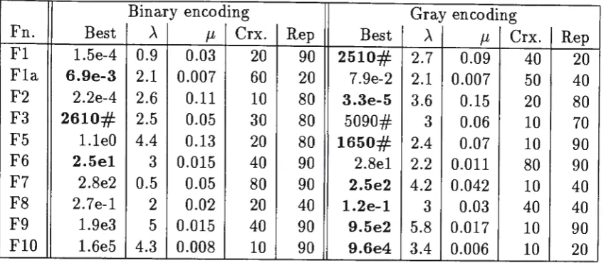
In Table 4,

">."

shows the Poissor1 mean which gave the best results in the Set 3 runs. "µ" gives the Poisson mean as a probability of bit mutation for the chromosome, assuming the chromosome is to undergo mutation.

Table 4: Results from Set 3 runs

Binary encoding _{Gray encoding}

Fn. Best .A µ Crx. Rep Best .A µ Crx. Rep

Fl 1.5e-4 0.9 0.03 20 90 2510# 2.7 0.09 40 20 Fla 6.9e-3 2.1 0.007 60 20 7.9e-2 2.1 0.007 50 40 F2 2.2e-4 2.6 0.11 10 80 3.3e-5 3.6 0.15 20 80 F3 2610# 2.5 0.05 30 80 5090# 3 0.06 10 70 F5 l.leO 4.4 0.13 20 80 1650# 2.4 0.07 10 90 F6 2.5el 3 0.015 40 90 2.8el 2.2 0.011 80 90 F7 2.8e2 0.5 0.05 80 90 2.5e2 4.2 0.042 10 40

F8 2.7e-l 2 0.02 20 40 1.2e-1 3 0.03 40 40

F9 1.9e3 5 0.015 40 90 9.5e2 5.8 0.017 10 90 FlO 1.6e5 4.3 0.008 10 90 9.6e4 3.4 0.006 10 20

Table 5: Results for 100% crossover and no mutation

Binary encoding Gray encoding Fn. Best Std D. Evals Best Std D. Eval. Fl 1.5e-2 2.8e-2 1670 6.le-2 le-1 2075 F2 2.4e-2 3.8e-2 4910 9.9e-2 le-1 4910 F3 2.4e0 l.2e0 2570 2.5e0 8e-l 3830 F5 2.5e0 3.3e0 2075 3.0eO 2.5e0 2075 F6 7.3el 1.8el 4910 8.4el l.4el 6152 F7 5.7e2 2.7e2 4910 7.7e2 2.5e2 3695 F8 7.3e0 3.5e0 6125 8.7e0 3.4e0 6125 F9 5.4e3 1.8e3 12,200 6.0e3 l.6e3 8555 FlO 6.3e5 l.le5 12,200 5.9e5 le5 16250

no mutation is used the progress of the GA stagnates and the column headed "Eval." indicates the number of evaluations after which no further improvement was made by the GA.

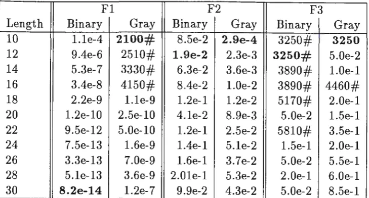
A set of runs to determine the effect of granularity on the performance of the GAs was also performed. These results are summarised in Table 6. The runs were performed for functions Fl, F2 and F3 and the length of representation for the function variables was varied from 10 to 30 bits.

Table 6: Varying gene length

Fl F2 F3

Length Binary Gray Binary Gray Binary Gray

10 1.le-4 2100# 8.5e-2 2.9e-4 _3250# 3250

12 9.4e-6 2510# 1.9e-2 2.3e-3 3250# 5.0e-2

14 5.3e-7 3330# 6.3e-2 3.6e-3 3890# 1.0e-1

16 3.4e-8 4150# 8.4e-2 1.0e-2 3890# 4460#

18 2.2e-9 l.le-9 l.2e-l 1.2e-2 5170# 2.0e-1

20 1.2e-10 2.5e-10 4.le-2 8.9e-3 5.0e-2 l.5e-l

22 9.5e-12 5.0e-10 l.2e-l 2.5e-2 5810# 3.5e-l

24 7.5e-13 l.6e-9 l.4e-l 5.le-2 1.5e-l 2.0e-1

26 3.3e-13 7.0e-9 l.6e-l 3.7e-2 5.0e-2 5.5e-l

28 5.le-13 3.6e-9 2.0le-1 5.3e-2 2.0e-1 6.0e-1

30 8.2e-14 l.2e-7 9.9e-2 4.3e-2 5.0e-2 8.5e-l

7

Discussion and Conclusions

7.1

Function Variables as Genes

Throughout this paper we have considered the fundamental unit of inheritance (genes) to be the function variables. This approach has enabled us characterise the effect of bit-flip mutation by probability distributions of changes in the function variables. This also showed the dependence of these changes on gene length ..

In Table 4, columns headed µ show the optimum bit-flip mutation rate, whereas the column headed

>.

shows the optimum gene mutation rate. The values for ,\ show much less variation. This indicates that the gene mutation rate is the more significant parameter.

7.2

Granularity

The results shown in Table 6 show the dramatic effect of granularity on GA performance. In general the best results are obtained with a coarse granularity; we believe that a fine granularity retards convergence by allowing only small changes in the variables with bit-flip mutation.

A glaring exception to this trend is shown in solving Fl using binary code representation where a finer granularity is preferable. A watch on the actual populations in this case shows that sometimes the population is trapped by a large Hamming cliff near the optimum (0,0,0). With a finer granularity, that particular cliff is closer to the origin and hence gives a better solution on these occasions.

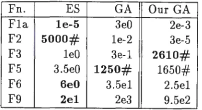
Table 7: Comparison of results with Hoffmeister and Back

Fn. ES GA Our GA

Fla le-5 3e0 2e-3 F2 5000# le-2 3e-5

F3 leO 3e-l 2610#

F5 3.5e0 1250# 1650# F6 6e0 3.5el 2.5el

F9 2el 2e3 9.5e2

For the functions Fla, F2, F6 and F9, the ES algorithm was significantly better, sometimes by several orders of magnitude. In these cases, our imple-mentation of the GA was superior to that of Hoffmeister and Back, narrowing the performance gap with ESs. And for F3 and F5 where the GA was superior to ES, our implementation was still superior.

It would appear that most of the superiority in our GA is due to the coarser granularity used. We made no effort here to optimise the granularity for perfor-mance, just selecting a granularity that was natural for the variable intervals in each case. So perhaps further improvements to the GA performance is possible by judicious selection of the representation length.

Of course it may be argued that these problems are artificial and that the optima occur at coordinates that can be represented using a coarse granularity. With "real" problems one would expect the optima to occur at fractional co-ordinates and a fine granularity would be needed to encompass such solutions. This suggests that the best performance with bit-flip mutation may be obtained ·

by starting with short representations and increasing the string lengths as the GA approaches an optimum. This approach has been tried by other researchers using delta coding and dynamic parameter encoding.

7 .3

Gray verses Binary Coding

7.4 The Nature of Mutation

Performance of our GAs are also affected by the number of genes (variables) in a chromosome that are allowed to mutate. Comparison of Tables 3

&

4 shows the value of optimising this. Note that the mean number of bits mutated for optimum performance, µ, varied greatly between the various functions. How-ever, the consequential mean number of genes mutated

(.A)

shows much less variation.

We have shown that when mutation and crossover are used as indepen-dent reproduction operators, that is a new chromosome is produced by either

crossover or mutation, best results are often obtained with quite low rates of

crossover and hence high rates of mutation (see Tables 2

&

3). This could indicate that the "explorative" nature of crossover is not needed for these func-tions, or that for these functions crossover is able to absorb quite high rates of introduced genes successfully. These results show that mutation is a very important operator for GAs, and should not be regarded as just an operator to replace allele values lost from the population.

References

Caruana, R, & Schaffer,

J.

D. 1988. Representation .and Hidden Bias: Gray vs. Binary Coding for Genetic Algorithms. In: Proceedings of the 5th International Conference on Machine Learning. pp. 153-161.

Davis, L. 1985. Job-shop Scheduling with Genetic Algorithms. In: Proceedings of an International Conference on Genetic Algorithms and their Applica-tions. pp. 136-140.

Davis, L. (ed). 1991. Handbook of Genetic Algorithms. Van Nostrand Reinhold.

Dawkins, R. 1982. The Extended Phenotype. Oxford University Press.

De Jong, K. A. 1975. An analysis of the behaviour of a class of genetic adaptive system. Doctoral dissertation, University of Michigan.

Falkenauer, E. A., & Delchambre, A. 1992. A Genetic Algorithm for Bin Packing and Line Balancing. In: Proceedings of 1992 IEEE International Confer-ence on Robotics and Automation(RA92). pp. 1186-1193.

Goldberg, David E. 1989. Genetic Algorithms in Search, Optimization B Ma-chine Learning. Addison-Wesley.

Gordon, V.S., & Whitley, D. 1993. Serial and Parallel Genetic Algorithms as Function Optimizers. In: Forrest, Stephanie ( ed), Proceeding of the Fifth International Conference on Genetic Algorithms. Urbana-Champain:

Morgan-Kaufmann. pp 177-183.

Evolution-Hoffmeister, F.,

&

Back, T. 1992 (Feb). Genetic Algorithms and Evolution

Strategies: Similarities and Differences. Technical Report No. SYS-1/92.

Systems Analysis Research Group, University of Dortmund, Germany.

Holland,

J.

H. 1992. Adaption in Natural and Artificial Systems. 2nd edn. MIT Press.

Hollstein, R. B. 1971. Artificial Genetic Adaption in Computer Control

Sys-tems. Ph.D. Dissertation, Department of Computer and Communication

Sciences, University of Michigan, Ann Arbor, Michigan.

Michalewicz, Z. 1994. Genetic Algorithms

+

Data Structures

=

Evolution

Pro-grams. 2nd edn. Springer - Verlag.

Rechenberg, R. 1973. Evolutionsstrategie: Optimierung technischer Syseme

nach Prinzipien der biologischen Evolution. Stuttgart:

Frommann-Holzboog.

Rosenbrock, H. H. 1960. An automatic method for finding the greatest or least value of a function. In: The Computer Journal. 3, vol. 3. pp 175-184.

Schwefel, H-P. 1977. Numerische Optimierung von Computer-Modellen mittels

der Evolutionsstrategie. Interdisciplinary systems research, vol. 26. Basel:

Birhauser.

Shekel,

J.

1971. Test functions for multimodal search techniques. In: Fifth

Annual Princeton Conference on Information Science and Systems.

Torn, A., & Zilinskas, A. 1989. Global Optimization. Lecture Notes in Computer Science, vol. 350. Springer-Verlag.