Cryptology ePrint Archive: Report2012/612. This is the full version of the article presented at ACISP 2013 under the same title. LNCS7959, pp.347–362. DOI:10.1007/978-3-642-39059-3_24
Analysis of the Non-Perfect Table
Fuzzy Rainbow Tradeoff
Byoung-Il Kim and Jin Hong
Department of Mathematical Sciences Seoul National University, Seoul 151-747, Korea
{samaria2,jinhong}@snu.ac.kr
Abstract. Time memory tradeoff algorithms are tools for inverting one-way functions, and they are often used to recover passwords from un-salted password hashes. There are many publicly known tradeoff al-gorithms, and the rainbow tradeoff is widely believed to be the best algorithm. This work provides an accurate complexity analysis of the non-perfect table version of the fuzzy rainbow tradeoff algorithm, which has not yet received much attention. It is shown that, when the pre-computation cost and the online efficiency are both taken into consider-ation, the non-perfect fuzzy rainbow tradeoff is preferable to the original rainbow tradeoff in many situations.
Keywords: time memory tradeoff, rainbow table, fuzzy rainbow, dis-tinguished point
1
Introduction
Cryptanalytic time memory tradeoff algorithms are tools for quickly inverting one-way functions with the help of pre-computed data. They are used by law enforcement agencies and hackers to recover passwords from unsalted password hashes, and the multi-target variants of the algorithms have been used [7, 10, 11, 15] to show that the GSM mobile phones are insecure.
There are a multitude of publicly known tradeoff algorithms. However, a search for password recovery tools on the Web reveals [1–4] that the rainbow tradeoff [23] is by far the most popular algorithm, and this seems to indicate that the rainbow tradeoff is widely believed, at least among implementers, to be the best tradeoff algorithm.
perfect distinguished point [12–14], and non-perfect distinguished point tradeoff algorithms, under typical situations, thus supporting the aforementioned beliefs. In this work, we analyze the execution behavior of the non-perfect table fuzzy rainbow tradeoff [6, 8], which has not yet received much attention. The results are then used to compare the performance of the fuzzy rainbow tradeoff against those of the usual perfect and non-perfect rainbow tradeoffs.
We find that, with the appropriate choice of parameters, the usual rainbow tradeoffs can achieve a certain degree of online efficiency that cannot be reached by the fuzzy rainbow tradeoff through any choice of its parameters. However, we also find that, for online efficiency levels that can be reached by both the fuzzy rainbow and usual rainbow tradeoff algorithms, the fuzzy rainbow tradeoff calls for less pre-computation effort than the usual rainbow tradeoffs. In other words, up to a certain point, for the same pre-computation investment, better online efficiency is returned by the fuzzy rainbow tradeoff. Since the massive pre-computation requirement stands as a significant barrier to any large scale deployment of the tradeoff technique, the fuzzy rainbow tradeoff will often be preferable to the original rainbow tradeoffs.
The main contribution of this article is in providing an accurate execution behavior analysis of the non-perfect table fuzzy rainbow tradeoff. The final part of this article, concerning algorithm comparisons, is mostly a careful application of the framework set by [19].
The fuzzy rainbow tradeoff is a combination of the distinguished point trade-off and the rainbow tradetrade-off. In fact, both the distinguished point and rainbow tradeoffs are special cases of the fuzzy rainbow tradeoff, corresponding to cer-tain extreme parameter choices. Hence, one might expect the performance of the fuzzy rainbow tradeoff to come somewhere in between those of the distin-guished point and rainbow tradeoffs. The findings of this paper, which indicate otherwise, could be seen as slightly surprising.
Arguments supporting the efficiency of the fuzzy rainbow tradeoff were given in the publications [6, 8] that introduced the algorithm. However, the argu-ments were based on the concept of hidden states, which totally disregards pre-computation cost, and the complexity claims made there were not tight enough to be accurate up to small constant factors. Since the performances of tradeoff algorithms often differ only by small constant factors, which nevertheless have heavy consequences in practice, it was not possible to provide an appropriate comparison of algorithms based on their results.
There are only two works concerning the fuzzy rainbow tradeoff, other than [6, 8], that we are aware of. The multi-target version of the fuzzy rainbow tradeoff is described as having been used during the presentation [21, 22] of a fully imple-mented attack on GSM phones, but no theoretical analysis was given there. The work [26] provides an entry-level analysis of the same algorithm, but incorrect assumptions were made concerning the parameters. Neither work mentions that the algorithm being dealt with appeared previously in [6, 8].
analyzing the execution behavior of the fuzzy rainbow tradeoff. Section 3 gives the probability of success, Section 4 gives the accurate online time complexity that takes the effects of false alarms into account, and Section 5 discusses the physical storage size required to record the pre-computation tables. The main parts of our arguments made during the analyses are experimentally verifying in Section 6. A method for fixing one fuzzy rainbow tradeoff parameter that is not used in other tradeoff algorithms is discussed in Section 7. Our theoretical findings are finally used in Section 8 to present a fair comparison between the fuzzy rainbow tradeoff and the usual rainbow tradeoffs. Concluding remarks are made in Section 9.
2
Preliminaries
The reader is assumed to be familiar with the basic tradeoff techniques. In this section, we fix the terminology and quickly recall the fuzzy rainbow tradeoff algorithm.
Throughout this paper, the one-way functionf :N → N is taken to act on a search space N of size N. The composition of the one-way function and the reduction function ofi-th color will be written asfi. The standard notation for
the number of chains per tablem, the chain lengtht, and the number of tablesℓ will be used. When dealing with DPs (distinguished points), the distinguishing property will always be assumed to be of probability 1
t, so that the expected
length of a random chain ist. The collection of allmchains, associated with one pre-computation table, is referred to as a pre-computation matrix.
The fuzzy rainbow tradeoff [6, 8] is a combination of the rainbow tradeoff and the DP tradeoff. Recall that each pre-computation matrix for the rainbow tradeoff containsmpre-computation chains, each of lengtht, that take the form
SP f1 −−→ ◦ f2
−−→ ◦ · · · ◦ ft
−−→EP, (1)
where SP and EP denote the starting and ending points, respectively. The color of the one-way function is changed at each iteration of the chain generation for a total of t different colors, for each matrix. An online chain for the rainbow tradeoff starts from one of the colors 1 ≤i ≤t and continues to the finalt-th color.
Also recall that each DP matrix containsm chains of variable lengths that take the form
SP fi
−−→ ◦ fi
−−→ ◦ · · · ◦ fi
−−→DP = EP, (2)
In the case of the fuzzy rainbow tradeoff, a distinguishing property and a positive integersare fixed, and pre-computation chains of the form
SP f1
−−→ ◦ · · · ◦ f1
−−→DP f2
−−→ ◦ · · · ◦ f2
−−→DP f3 −−→ ◦ · · ·
· · · fs−1
−−−−→DP fs
−−→ ◦ · · · ◦ fs
−−→DP = EP (3)
are used. The colored one-way function iterations are continued under a fixed color until a DP is reached, after which the iterations are continued with a different color. A total of s colors are used for each pre-computation chain, so that the average chain length becomests. An online chain for the fuzzy rainbow tradeoff starts from one of the colors 1≤i≤sand terminates at the DP for the finals-th color.
As with other tradeoff algorithms, in the pre-computation phase of the fuzzy rainbow tradeoff,mchains are generated for each of theℓpre-computation tables, and only the starting point and ending point pairs, sorted according to the ending points, are stored in the pre-computation tables.
The algorithm we have just described is the non-perfect table version of the fuzzy rainbow tradeoff. One can also consider the perfect tables version of this algorithm, obtained by retaining just one chain from every set of merging chains. However, only the non-perfect table version of the fuzzy rainbow tradeoff will be studied in this work. The perfect table version is likely to be more efficient during the online phase, but will require higher pre-computation cost. The results of this paper indicate that the perfect table fuzzy rainbow tradeoff is well worth analyzing, and this will be a subject of our future study.
The fuzzy rainbow tradeoff analogue of the matrix stopping rules ismt2s≈ N. In other words, we always assume that the parametersm,t, ands, for the fuzzy rainbow tradeoff, are chosen in such a way that the matrix stopping constant Fmsc = mt2s
N is neither too large nor very close to zero. We shall often express
such a condition simply asFmsc=Θ(1). Appropriateness of the matrix stopping rule mt2s
≈Nis explained in [6]. The theoretical arguments of this paper will be easier to comprehend when s is assumed to be much smaller than m or t, even though no such assumption appears in [6, 8]. It will later become clear that thesvalues of interest will mostly be in the range 15∼100.
To complete the description of the fuzzy rainbow tradeoff algorithm, the order of online chain creation needs to be clarified. In short, all the tables are processed in parallel, in the sense that the usual rainbow tradeoff processes tables in parallel.
Just as with the usual rainbow tradeoff, in real implementations, theℓonline chains may or may not be generated simultaneously. It suffices to have all of them generated and all the associated alarms treated, in any order, before moving onto the next pass. Our theoretical arguments are placing a slight disadvantage on the fuzzy rainbow tradeoff by assuming the full processing of any single pass that has started, but our results will still be good approximations of the true situation, as long assis not too small.
The fuzzy rainbow tradeoff algorithm introduced by [6, 8] was a time mem-ory data tradeoff algorithm that aimed to invert just one of multiple inversion targets. Since it is known [9] that the multi-target application of the original rainbow tradeoff results in a tradeoff curve that is quite inferior to those of the multi-target classical Hellman or distinguished point tradeoffs, the inten-sion of [6, 8] was to create a variant of the rainbow tradeoff with a multi-target tradeoff curve of theT M2D2
≈N2form. However, in this work, we will restrict ourselves to theD= 1 case and treat the fuzzy rainbow tradeoff as a single target inversion algorithm. The multi-target version of the fuzzy rainbow tradeoff must be compared against the multi-target versions of the classical Hellman and DP tradeoffs, but nothing similar to [19, 20] has yet appeared for these multi-target algorithms. Furthermore, preliminary analysis seems to indicate that the analy-ses for the single target inversion algorithms will carry over to the multi-target algorithms almost word for word.
The fuzzy rainbow matrix may be viewed as a concatenation ofs DP sub-matrices, with the ending points of one DP sub-matrix used as the starting points for the next DP sub-matrix. Throughout this work, thei-th (1≤i≤s) DP sub-matrix will be denoted by DMi. The only difference between DMi and a normal non-perfect DP matrix is thatDMimay contain duplicate starting points, that bring about fully identical chains.
Any implementation of a tradeoff algorithm that relies on DPs will set a chain length bound to detect chains falling into loops. In this work, we assume that a sufficiently large chain length bound is used. This is not exactly equivalent to taking the limit where the chain length bound is sent to infinity. A more detailed discussion of the exact meaning of this assumption may be found in [19, 20].
There will be many approximations made throughout this paper. Most of these will depend on the relation (1− 1
b) a
≈ e−ab, which is appropriate when
a = O(b). A more precise statement can be found in [19]. Under any reason-able choice of tradeoff parameters, these approximations will be very accurate whenever we apply the relation, and they will be written as equalities rather than as approximations. Another class of approximations appearing in this pa-per will involve interpretation of finite sums as definite integrals. Once again, when the summation is made over a large index set so that the approximation is accurate, we shall silently write the relation as an equality rather than as an approximation.
3
Probability of Success
The number of one-way function invocations required to construct all the pre-computation tables is expected to be mtsℓ. Let us define the pre-computation coefficient of the fuzzy rainbow tradeoff that uses parametersm, t, s, andℓ to be
Fpc= mtsℓ
N , (4)
so that, when the effort of table sorting, which is of much smallermℓlogmorder, is ignored, we may state FpcNas the cost of pre-computation.
We also define thecoverage rate of a fuzzy rainbow matrix to be Fcr=
1
mts |DM1|+|DM2|+· · ·+|DMs|
, (5)
where |DMi| denotes the number of distinct points expected in thei-th DP sub-matrix. Readers familiar with the definitions of the coverage rate appearing in previous works should note the slight difference. The current definition does not refer to the total number of distinct points in the pre-computation matrix. Nev-ertheless, the following proposition shows that the above is the natural definition to use in the case of fuzzy rainbow tradeoffs.
Proposition 1. Given an inversion target created from a random input to the one-way function, the fuzzy rainbow tradeoff will succeed in recovering the correct input with probability
Fps= 1−e−
FcrFpc
.
Proof. The probability of successful inversion expected from the single DP sub-matrixDMi is |
DMi|
N . Since the DP sub-matrices that were created with different
reduction functions can be treated as being independent, the success rate of the complete online phase is
Fps= 1−
s
Y
i=1
1−|DMi|
N
ℓ
.
This may be approximated by
Fps = 1−
s
Y
i=1
exp−|DMi|ℓ
N
= 1−exp−
s
X
i=1 |DMi|
ℓ
N
= 1−exp−Fcrmtsℓ N
= 1−exp −FcrFpc
,
as claimed. ⊓⊔
These different versions of the inversion problem behave sufficiently differently to require separate analyses, if the accuracy aimed for by this paper is to be obtained. A more careful definition of |DMi|, suitable for the inversion problem
considered in this work, would have counted only the points that were used as inputs to the one-way function during the pre-computation, disregarding the ending points. Careful treatment of these technical details, which we do not illustrate fully in the remainder of this paper, can be found in [19].
To utilize the above proposition, we need a way to express the coverage rate in terms of the tradeoff algorithm parameters. Recall from [18, 20] that the number of distinct entries|DM|contained in a non-perfect DP matrix satisfies
|DM|=mept, (6)
wheremep denotes the number of distinct ending points of the DP matrix. The work [20] uses this fact in conjunction with another expression for |DM|, found in [19], to obtain the formula
mep=msp
2 1 +
q
1 +2mspt2
N
, (7)
that relates the number of distinct starting pointsmsp to the number of distinct ending pointsmep in a normal DP matrix.
Returning to the fuzzy rainbow matrices, let us usemi−1 andmi to denote
the number of distinct starting points and ending points, respectively, expected in each DP sub-matrix DMi. In particular,m0 =m andms are the numbers of
distinct starting and ending points, respectively, of the full fuzzy rainbow matrix. We shall refer to each collection ofmi points as thei-thcolor boundary points
of a fuzzy rainbow matrix, where 0≤ i ≤s. Adopting the above two facts to our situation, we can state that
|DMi|=mit (8)
and
mi+1=mi
2 1 +
q
1 + 2mit2 N
with m0=m (9)
are to be expected at each applicable color indexi. The following closed-form formula formi is easier to utilize than the iterative formula (9).
Lemma 1. When the number of colors s used in each pre-computation table is large, the number of i-th color boundary points in a fuzzy rainbow matrix is expected to be
mi=
2m 2 +Fmscis
,
Proof. The iterative formula (9), written in a series expansion form, is
mi+1=mi
1−1 2
mit2
N
+Omi
mit2
N
2
.
Since the lemma statement assumes mit2
N =O
1
s
to be small, we can ignore the big-O part and rewrite this as the difference equation
mi+1
m −
mi
m =− Fmsc 2s mi m 2 .
As an application of the Euler method, we can interpret this as the differential equation
y′ =−F2smscy2, with the initial conditiony(0) =m0
m = 1, and solve foryto obtain
mi
m = 2 2 +Fmscis
,
which is the claimed formula. ⊓⊔
The coverage rate, at least for the larges values, follows directly from this lemma.
Proposition 2. When the number of colorssused in each pre-computation table is large, the coverage rate is
Fcr= 2 Fmsc
ln1 +Fmsc 2
for a single fuzzy rainbow matrix.
Proof. Combining Lemma 1 and (8), one can check that
Fcr= 1 mts
s
X
k=1 |DMk|=
1 s s X k=1 mk m = s X k=1 2 2 +Fmscks
1 s =
Z 1
0 2 2 +Fmscu
du.
Computation of the final definite integral results in what is claimed. ⊓⊔ The computation done in this proof also gives the partial coverage rate
1 mts
s
X
k=i+1 |DMk|=
1 s
s
X
k=i+1 mk
m = 2 Fmscln
2 +Fmsc
2 +Fmscsi
, (10)
which contains Proposition 2 as the special case ofi= 0.
method used in Lemma 1 and the second being the interpretation of a summa-tion an a definite integral. However, as explained below, one can verify through explicit computations that formula (10) is accurate even whensis very small.
After rewriting (9) in the form mi+1
m =
mi
m
2 1 +q1 + 2Fmsc
s mi
m
with m0
m = 1, (11)
one can iteratively compute all mi
m, for any givenFmscand anysthat is not too
large. In Figure 1, we have compared
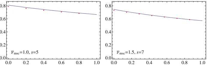
Fmsc=1.0, s=5
0.0 0.2 0.4 0.6 0.8 1.0
0.0 0.2 0.4 0.6 0.8
Fmsc=1.5, s=7
0.0 0.2 0.4 0.6 0.8 1.0
0.0 0.2 0.4 0.6 0.8
Fig. 1.Comparisons between closed-form formula (line) and iteratively computed val-ues (dots) of the partial coverage rate at smalls. (x-axis:i
s;y-axis: s s−i
Ps k=i+1
|DMk| mts)
s s−i×
1 s
s
X
k=i+1 mk
m, (12)
with mk
m iteratively computed through (11), against the graphs of
s s−i×
2 Fmscln
2 +Fmsc
2 +Fmscis
, (13)
at very smallsvalues. The s
s−i factor has been multiplied to the partial coverage
rates so that all values are close to 1 and they may be gather within a single figure. The figures testify that Lemma 1, Proposition 2, and formula (10) are accurate even at these very small s values. Since it will become clear, later in Section 7.3, that thesvalues of interest will be somewhat larger than those given by these explicitly computed examples, henceforth, we shall treat Lemma 1, Proposition 2, and formula (10) as being valid for allsvalues of interest.
Remark 1. Proposition 1 implies that any set of parametersm,t,s, andℓ that achieves the success rateFps must satisfy the relation
ℓ t =
Fpc Fmsc =
{−ln(1−Fps)}
and Proposition 2 gives the coverage rate Fcr as a function of the single vari-ableFmsc. Hence, when parameter sets are restricted to those that achieve a fixed requirementFps on the success rate, the ratio ℓ
t may also be seen as a function
of the single variableFmsc.
Remark 2. Recall that we are working with parameters for whichFmscis ofΘ(1) order. This fact and Proposition 2 imply that the coverage rate
Fcr= 1−1 2
Fmsc
2
+1 3
Fmsc
2
2
−14Fmsc2 3+· · ·
is also ofΘ(1) order. Hence, unless the success rate requirementFps is unrealis-tically close to 100%, relation (14) implies thatℓandt are of similar order.
4
Online Complexity
Having secured full knowledge concerning the success rate of the fuzzy rainbow tradeoff, we next discuss the online execution complexities. Our interest lies with the average case complexity, rather than the worst case complexity.
We first write the probability for each pass of the online phase to be executed. Lemma 2. For any number of colorssof interest, the probability for the online chains that start from the i-th colors of the fuzzy rainbow matrices to be gener-ated, i.e., the probability for the DP sub-matrices DMi within the fuzzy rainbow
matrices to be searched for the correct answer to the inversion problem, is
2 +Fmsci
s
2 +Fmsc
2ℓt
.
Proof. The online chains that start from the i-th color of any fuzzy rainbow matrix will be generated if and only if the correct answer to the inversion target does not belong to the DP sub-matricesDMi+1, . . . ,DMscontained in theℓfuzzy
rainbow matrices. Hence, the probability under consideration is
s
Y
k=i+1
1−|DMk|
N
ℓ
= exp− ℓ
N
s
X
k=i+1 |DMk|
= exp−ℓtFmsc
s
X
k=i+1 |DMk|
mts
=2 +Fmsc
i s
2 +Fmsc
2ℓt
,
where the final equality follows from (10), which hold true for all s values of
interest. ⊓⊔
Proposition 3. For any number of colors s of interest, the generation of the online chains during the online phase of a fuzzy rainbow tradeoff is expected to require
tℓ
s
X
i=1
(s−i+ 1)2 +Fmsc
i s
2 +Fmsc
2ℓt
iterations of the one-way function.
Proof. Each of the ℓ online chains that start from the i-th color of each fuzzy rainbow matrix is expected to require (s−i+ 1)t iterations of the one-way function. The probability for each of these iterations to be executed is given by Lemma 2. The claim is a simple combination of these two observations. ⊓⊔ Our next objective is to express the cost of dealing with alarms, which is the remaining component of the online time complexity. To compute the cost of resolving alarms associated with an online chain that starts from thei-th color, the merging of normal single colored DP chains needs to be considered first. Lemma 3. The probability for two randomly generated DP chains to merge into each other is t2
N.
Proof. Assuming t ≪ √N, the probability for the first chain to become a DP chain of lengthiis 1−1
t
i−1 1
t. The probability for the second chain to merge
into this chain at itsj-th iteration is 1−1
t− i+1
N
j−1i+1
N . Hence, the probability
for two chains to merge can be expressed as ∞
X
i=1 1−1
t
i−11
t ∞
X
j=1 1−1
t − i+ 1
N
j−1i+ 1
N .
The two infinite sums here should be understood as expressing the summations up to a sufficiently large chain length bound, so that we have i+1
N ≪
1
t and
1−1
t − i+1
N
j−1
≈ 1−1
t
j−1
. The above may now be approximated by t2 N Z ∞ 0 Z ∞ 0
e−ue−vu dv du= t 2
N,
and this completes the proof. ⊓⊔
With the simplifying assumption that the two DP chains are of lengtht, the merge probability can be computed more simply as
1−1− t
N t =t 2 N − t 2 t N 2
+· · · −(−1)t
t t t N t ≈t 2
N, (15)
and it was unclear as to whether this fact could bring about a difference in the final expression for the merge probability, when averaged over all chain lengths. The merge probability for single colored chains is now used to compute the cost of resolving alarms from the fuzzy rainbow chains.
Lemma 4. Consider a single fuzzy rainbow pre-computation matrix and its as-sociatedscolors. Assume the generation of an online chain for this matrix that starts from the i-th color. The cost of resolving alarms that may be induced by possible merges of this online chain with the chains of the single fuzzy rainbow matrix is expected to be
tFmsc s
i(s−i+ 1) + 1
iterations of the one-way function.
Proof. The alarms need to be handled separately for each pre-computation chain that merges with the online chain. The resolving of an alarm associated with one pre-computation chain requires the same amount of work regardless of whether or not the pre-computation and online chains merge with other pre-computation chains. Hence, the total cost of resolving alarms is mtimes the cost associated with one pre-computation chain. Below, we will focus on the possible merge be-tween the online chain and a single randomly generated pre-computation chain. If the online chain that starts from the i-th color merges with a given pre-computation chain, the merge will be at precisely one of the colorsi,i+ 1, . . . , s. The case of possible merge at the i-th color will be treated separately from the possible merge at strictly later colors.
The probability for the i-th colored DP sub-chain of the pre-computation chain to be of length pis 1−1
t
p−1 1
t. The probability for the online chain to
merge into this DP sub-chain of lengthpwithin its i-th color DP sub-chain is ∞
X
q=1
1−1 t −
p+ 1
N
q−1p+ 1
N =
p+ 1
N
1 1
t + p+1
N
≈ t(p+ 1)
N .
To resolve the alarm from such a merge, one must expect to compute (i−1)t iterations of the one-way function to regenerate the pre-computation chain up to the start of thei-th colored sub-chain and then additionally computepiterations to reach the end of the i-th colored sub-chain. The only exception is when the correct answer is found, but this is a single rare event among the many alarms, and can be ignored. Hence, the cost of resolving an alarm that may occur due to a possible merge at thei-th color is
∞
X
p=1
1−1 t
p−11
t ·
t(p+ 1)
N ·
(i−1)t+p ,
which may be approximated by t3
N
Z ∞
0
e−uu(i−1) +u du= (i+ 1)t 3
For color indicesj > i, we can infer from Lemma 3 that the merge of the two chains at thej-th color will occur with probability 1−t2
N
j−i t2
N. The combined
probability of merge at any one of the colors appearing strictly after the i-th color is
s
X
j=i+1
1−t 2
N
j−it2
N =
1−t 2
N
n
1−1−t 2
N
s−io
≈(s−i)t 2
N.
The final approximation is true since t2
N ≪1, and the same result would have
been obtained if we had simply treated the merge probability at each color to be t2
N, regardless of j. Since any such merge will require justititerations of the
one-way function to resolve, the sum of costs associated with possible merges at all colors appearing strictly after thei-th color is
(s−i)t 2
N ·it.
The sum of the two computed costs (i+ 1)t
3
N+i(s−i)
t3
N =
i(s−i+ 1) + 1 t 3
N
is the cost expected from a single pre-computation chain, andmtimes this value
is what is claimed. ⊓⊔
In the case of the DP tradeoff, the cost of resolving alarms can be reduced slightly [18] through the online chain record (OCR) technique [17, 24]. The method is to keep a full record of the online chain during its generation, so that any pre-computation chain regeneration can be stopped at the exact point of merge, rather than at the terminating DP. Some readers may have wondered why the OCR technique is not being applied to the fuzzy rainbow tradeoff. A careful reading of the above proof shows that, for an online chain that starts from thei-th color, the OCR technique can take effect only if the merge occurs within thei-th colored sub-chain. This observation indicates that the application of OCR technique to the fuzzy rainbow tradeoff will reduce the number of one-way function iterations, at the inconvenience of more frequent memory accesses, but the reduction will be too small to be of interest, unless a very smallsis in use.
During the online phase, the generation of an online chain that starts from thei-th color, which the above lemma assumes, is done only if all previous shorter online chains have failed to return the correct answer. The following statement accounts for this in computing the cost of resolving alarms.
Proposition 4. For any number of colorss of interest, the resolving of alarms during the online phase of a fuzzy rainbow tradeoff is expected to require
tℓFmsc s
s
X
i=1
i(s−i+ 1) + 1 2 +Fmsc
i s
2 +Fmsc
2ℓt
Proof. The probability for the online chains that start from the i-th colors of the pre-computation matrices to be generated is given by Lemma 2. The cost of alarm treatment expected from each of these online chains is stated by Lemma 4. It now suffices to multiply by ℓ to account for the multiple online chains and sum the product of the mentioned probability and expected work over all color
indices. ⊓⊔
The two components of the online time complexity for the fuzzy rainbow tradeoff have been obtained, and we are ready to state the tradeoff coefficient, which succinctly expresses the online efficiency of a tradeoff algorithm.
Theorem 1. For any number of colors sof interest, the time memory tradeoff curve for the non-perfect table fuzzy rainbow tradeoff is T M2=F
tc,sN2, where
the tradeoff coefficient is
Ftc,s=F2msc
ℓ
t
3Xs
i=1
1−i−1 s
1 +Fmsc i s
+Fmsc s2
2 +Fmsci
s
2 +Fmsc
2ℓt1
s.
Proof. The storage complexity of the fuzzy rainbow tradeoff is M = mℓ, and the time complexity is the sum
T =tℓ
s
X
i=1
n
(s−i+ 1)Fmsc i s+ 1
+Fmsc s
o2 +Fmsci
s
2 +Fmsc
2ℓt
of the two terms given by Proposition 3 and Proposition 4. The tradeoff curve is obtained by appropriately combining the two complexities M and T. Easy modifications of the formula are needed to arrive at the form of the tradeoff
coefficient presented by this theorem. ⊓⊔
Remark 3. Note that the time complexityT, appearing in the above proof, can be bounded from below by
T ≥tℓ
s
X
i=1
(s−i+ 1) 2 2 +Fmsc
2ℓt
=tℓs(s+ 1) 2
2
2 +Fmsc
2ℓt
and bound from above by
T ≤tℓ
s
X
i=1
n
(s−i+ 1)(Fmsc+ 1) + Fmsc
s
o
=tℓns(s+ 1)
2 (Fmsc+ 1) +Fmsc
o
.
Since we know from Remark 2 that ℓ =Θ(t), the online time complexityT of the fuzzy rainbow tradeoff must be ofΘ(t2s2) order. In fact, one can similarly verify from Proposition 3 and Proposition 4 that both the online chain creation and alarm resolving consumesΘ(t2s2) iterations of the one-way function.
very implementation dependent. Since, when the pre-computation tables reside in fast memory, the cost of table lookups could be negligible in comparison to the cost of one-way function computations, table lookups are mostly ignored in theoretical analyses of the tradeoff algorithms. The same approach will be taken by this paper and the result below will not be referred to in the rest of this paper. However, in practice, table lookups can become a bottleneck and affect the performance of the algorithms significantly.
Proposition 5. For any number of colorss of interest, the online phase of the fuzzy rainbow tradeoff is expected to call for
ℓ
s
X
i=1
2 +Fmsci
s
2 +Fmsc
2ℓt
,
table lookups.
Proof. The probability for the online chains that start from thei-th colors of the pre-computation matrices to be generated is given by Lemma 2, and every such online chain generation will call for a single table lookup per pre-computation table. Hence, the expected number of lookups can be written as claimed. ⊓⊔
Remark 4. The table lookup count stated by this proposition is upper bounded bysℓand lower bounded bysℓ 2
2+Fmsc
2ℓt. Referring to Remark 2 one more, we
can state that the number of table lookups made by the online phase of the fuzzy rainbow tradeoff is ofΘ(ts) order.
Later discussions in Section 8 show that ts for the fuzzy rainbow tradeoff corresponds naturally to t for the usual rainbow tradeoff, in a manner that is somewhat analogous to how mtfor the classical Hellman tradeoff corresponds tomfor the rainbow tradeoff. Since the usual rainbow tradeoff requiresΘ(tℓ) = Θ(t) table lookups [19], the table lookup requirements of the fuzzy rainbow and original rainbow tradeoffs are comparable.
5
Storage Optimization
The storage complexityM appearing in the tradeoff curve of Theorem 1 refers to the total number of entries, i.e., starting and ending point pairs, that are written to the pre-computation tables. In practice, the physical storage size, which depends not only on the number of table entries, but also on how many bits of storage must be allocated to each table entry, will be more important.
The issue of recording the ending points effectively is more complicated. There are three major techniques that can be used with various tradeoff algo-rithms. Slightly more detail than what is explained below can be found in [19, 20]. The first of the three methods is the index file method [11], which is widely used even outside the tradeoff subject. Once a pre-computation table has been sorted according to the ending points, two consecutive ending points in the table are highly likely to share a small number of common significant bits. This predictability of the significant bits can be used to remove almost logmbits per table entry, without any loss of information concerning the ending points, when the table containsmentries. A generalization of this storage technique is widely known by the name of hash tables.
The second method for reducing ending point storage size is applicable only when the ending points are DPs. One simply does not have to record any por-tion of the ending points that can be recovered from the distinguishing prop-erty [11, 25]. This allows removal of logtbits from each ending point without any information loss, when the distinguishing property is of 1
t probability. Clearly,
the fuzzy rainbow tradeoff allows application of this technique.
The final technique is to simply truncate the ending points to a certain length before recording them to storage [8, 11]. During the online phase, the terminating DP of an online chain is likewise truncated before being searched for in the pre-computation table. This reduces the storage requirement, but since partial matches of ending points will now be incorrectly announced as collisions, this will cause a new type of false alarms to appear and increase the cost of resolving alarms. In the remainder of this section we work to find the degree of truncation that restricts the side effects of ending point truncation to a negligible fraction of the online time complexity.
Let us assume a fixed truncation method for the ending points with a trun-cated match probability of 1
r. That is, we assume that the truncated outcome of
two independently and randomly chosen ending points, which are a priori DPs, will be identical with probability 1
r. For example, the case of no truncation
cor-responds to 1
r = t
N. In most cases, the truncated match probability of
1
r can be
obtained by retaining just logr bits of each ending point, that are unrelated to the distinguishing property. Note that whether the part that can be recovered from the distinguishing property, which contains no entropy, is also retained, does not affect the truncated match probability.
The extra cost incurred by the truncation-related alarms is stated below. Proposition 6. Assume the use of the ending point truncation method with the truncated match probability set to 1
r. Then, during the online phase of the fuzzy
rainbow tradeoff, one can expected to observe
tℓm r
s
X
i=1
i2 +Fmsc
i s
2 +Fmsc
2ℓt
Proof. As was argued during the proof of Lemma 4, it suffices to focus on the possible merges between a set ofsonline chains starting at different colors and a single pre-computation chain, and later account for multiple pre-computation chains.
We first need to separate the normal alarms from alarms caused by end-ing point truncations. Consider an online chain that starts from the i-th color. Through an argument similar to that appearing in the proof of Lemma 4, we can deduce from Lemma 3 that the probability for the online chainnotto merge into any single fixed pre-computation is 1−(s−i+ 1)t2
N. Unless
1
r ≈ t
N, the
probability for the non-merging two chains to bring about a truncated match is 1
r. Hence, the probability for an online chain that starts from thei-th color to
cause a truncation related alarm is
n
1−(s−i+ 1)t 2
N
o1
r.
Each of these pseudo-alarms will requireititerations of the one-way function to resolve. Taking the ℓm pre-computation chains into account and recalling Lemma 2, which gives the probability for an online chain that starts from the i-th color to be generated, the cost of dealing with truncation-related alarms can be written as
ℓm
s
X
i=1
it·n1−(s−i+ 1)t 2
N
o1
r·
2 +Fmsci
s
2 +Fmsc
2ℓt
.
It now suffices to observe that (s−i+ 1)t2
N =O
1
m
to realize that the claimed
formula is an accurate approximation. ⊓⊔
The cost stated by this proposition is upper bounded by
tℓm r
s
X
i=1
i=tℓm r
s(s+ 1) 2 and lower bounded by
tℓm r
s
X
i=1
i1−t 2s
N
2
2 +Fmsc
2ℓt
≈tℓm r
s(s+ 1) 2
2 2 +Fmsc
2ℓt.
Recalling Remark 2, given at the end of Section 3, we can state that the added cost of dealing with truncation-related alarms is ofΘ t2s2m
r
order. In compar-ison, Remark 3 states that the time complexityT is ofΘ(t2s2) order.
The two time complexity orders imply that, if m
r is a sufficiently small
Of course, if the truncated ending points still contain bits that can be re-covered from the DP definition they may also be removed without any loss of information. Furthermore, even the remaining effective logmbits of the ending points can mostly be removed through the index table method, without any loss of information.
In summary, storage of each starting point of the fuzzy rainbow tradeoff requires logm bits and the storage of each ending point requires a very small number ε of bits. Each entry of the fuzzy rainbow tradeoff can be recorded in logm+εbits.
Now that we have seen the detailed effects of the ending point truncation method, we can present an overall interpretation of the inner workings that is easier to understand. The cost of resolving alarms is ofΘ(t2s2) order (Remark 3) and each alarm induces Θ(ts) iterations of the one-way function, on average. Hence, one is expected to encounterΘ(ts) alarms during the online phase. Since this is also the approximate number of table lookups expected during the online phase (Remark 4), one can conclude that each table lookup incursΘ(1) alarm, or merges between an online chain and a pre-computation chain, on average. Hence, as long as slightly more than logmbits of each ending point are retained, so that the ending points within any single pre-computation table remain distinguishable from each other and also from the truncated online chain ending point, the number of pseudo-collisions will be kept at a small fraction of the Θ(1) order true merges.
6
Experimental Results
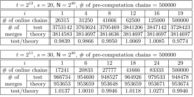
A small number of the chains did not reach a DP within our chain length bound of 15t, at various colors, and were prematurely discarded. A total of ten fuzzy rainbow matrices were generated, and the number ofi-th color boundary points was averaged separately for eachi.
Table 1.Number of color boundary points mi
m in a fuzzy rainbow matrix for a smalls. (m= 2000,t= 213
,s= 7,N= 240 )
i 0 1 2 3 4 5 6 7
test 1.0000 0.9457 0.8955 0.8494 0.8094 0.7743 0.7419 0.7119 Eq. (11) 1.0000 0.9454 0.8964 0.8521 0.8119 0.7752 0.7416 0.7108 Lemma 1 1.0000 0.9425 0.8912 0.8452 0.8038 0.7662 0.7320 0.7007
Test results for the smalls= 7 case is given in Table 1. It is clear that the experimental data is very close to the original theoretical values given by the iterative formula (11). This justifies our treatment of each DP sub-matrix DMi
as a normal DP matrix that contains a predictable number of duplicate starting points or chains. The main target of verification, which is the closed-form formula for mi
m given by Lemma 1, outputs numeric values that are slightly further away
from the experimental data, but the error is by less than 2% at the worst.
m=3000, t=212, s=20,N=240
Fmsc=0.92
0.0 0.2 0.4 0.6 0.8 1.0
0.0 0.2 0.4 0.6 0.8 1.0
m=12000, t=211, s=30,N=240
Fmsc=1.37
0.0 0.2 0.4 0.6 0.8 1.0
0.0 0.2 0.4 0.6 0.8 1.0
Fig. 2.Number of color boundary points in a fuzzy rainbow matrix (line: theory;dots: test;x-axis: i
s;y-axis: mi
m)
Our second experiment is designed to verify our arguments concerning the cost of resolving alarms. There are two main components to this argument. The first component is the probability for the online chains that start from thei-th color to be generated. This is tightly connected to the partial coverage rate formula (10), which has already been tested indirectly through our first experiment.
The second major component of the alarm cost argument is a technical claim made during the proof of Lemma 4. It concerns the probability of merge between a pre-computation chain and an online chain that starts from the i-th color. Explicitly, we had stated the combined probability of such merges at any one of the colors appearing strictly after thei-th color as (s−i)t2
N.
The experimental verification of this claim was carried out as follows. Multi-ple pre-computation chains were generated, and their color boundary DPs were recorded, rather than just their ending points. Since we were treating these chains as individual computation chains, rather than as members of a pre-computation matrix, no sorting was done. After fixing a starting color index i, online chains were generated to the ending points. The first DP of the online chain, i.e., the DP that ends the i-th colored sub-chain, in addition to the ter-minating DP, were recorded. For each online chain, we did a linear search over the collection of pre-computation chains for matching ending points. Whenever a collision was found, we compared the first DP of the online chain against the corresponding color boundary DP of the colliding pre-computation chain to check whether the merge occur within the i-th color sub-chain or strictly after thei-th color, and occurrences of only the latter type of collisions were counted. Online chains that start at different color indices were tested for merges against a common large collection of pre-computation chains.
Since the matrix stopping rule plays no role in this experiment, we were free to use any large number of pre-computation chains, and test repetitions were not necessary. Two sets of tests, corresponding to different parameter choices, were executed.
The experimental results are summarized in Table 2. The theoretical merge counts listed in the table were computed by multiplying the number of pre-computation chains and the number of online chains generated for the indexito the claimed probability (s−i)t2
N. Larger number of chains were used when
test-ing shorter online chains, since merges are seen less often with these chains, and a smaller number of merges would bring about unreliable data. The experimen-tally obtained merge counts for the two sets of tests are close to our theoretical predictions.
7
Number of Colors
s
Table 2.Probability of merge between an online chain that starts from thei-th color and a pre-computation chain. For each test setting, the number of merges at colors strictly after thei-th color are listed.
t= 212
,s= 20,N= 240
, # of pre-computation chains = 500000
i 1 4 8 12 16 19
# of online chains 26315 31250 41666 62500 125000 500000 # of
merges
test 3753142 3763624 3795469 3841206 3847142 3728423 theory 3814583 3814697 3814636 3814697 3814697 3814697 test/theory 0.9839 0.9866 0.9950 1.0069 1.0085 0.9774
t= 211
,s= 30,N= 240
, # of pre-computation chains = 500000
i 1 6 12 18 24 29
# of online chains 17241 20833 27777 41666 83333 500000 # of
merges
test 966734 954600 948527 964926 979533 948478 theory 953653 953659 953648 953659 953671 953674 test/theory 1.0137 1.0010 0.9946 1.0118 1.0271 0.9946
infinite family of algorithms indexed by the positive integers, and compare the performances of these multiple algorithms against each other.
7.1 The Fpc versusFtc Curve
To carry out the performance comparisons as suggested by [19], we need to draw the Fpc versus Ftc,s curves for the fuzzy rainbow tradeoff, under various fixed
Fps and s values. The analyses given in the previous sections contain all the information required for this task, and let us briefly explain how to utilize this information to explicitly plot the curves.
Recall from Remark 1, given at the end of Section 3, that both the coverage rate Fcr and the ratio ℓt may be seen as functions of the single variable Fmsc, when parameters are restricted to those that achieve a fixed success rate. Hence, given any fixeds, we may view both the pre-computation coefficient
Fpc= {−ln(1−Fps)} Fcr
(16) and the tradeoff coefficientFtc,sof Theorem 1 as functions of the single
parame-terFmsc, when under a fixed success rate requirementFps. Given anyFps ands, theFpc versusFtc,s curve can be drawn as a curve parameterized byFmsc.
It will become evident in the next subsection that thesvalues of interest are in the range 15∼100. Hence, the summation appearing in the formula forFtc,s
does not bring about any practical difficulties in handling of the formulas, for example, in drawing the curves or finding the lowest point on each curve.
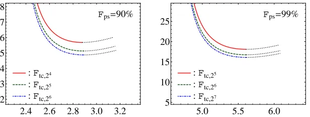
Example curves are presented in Figure 3. In each box, thex-axis gives the pre-computation coefficientFpcand they-axis gives the tradeoff coefficientsFtc,s.
:Ftc,24 :Ftc,25 :Ftc,26
Fps=90%
2.4 2.6 2.8 3.0 3.2
2 3 4 5 6 7 8
:Ftc,25 :Ftc,26 :Ftc,27
Fps=99%
5.0 5.5 6.0
5 10 15 20 25
Fig. 3. The tradeoff coefficients Ftc,s in relation to their respective pre-computation costs, at smalls(x-axis: pre-computation coefficient;y-axis: tradeoff coefficient).
closer to the left edge correspond to smaller pre-computation requirements. An implementer that wishes to utilize optimal online efficiency, at all costs, will choose to work with parameters corresponding to the lowest point of a curve, while an implementer with only modest pre-computation resources will have to be satisfied with a point that is situated higher but closer to the left edge. However, any set of parameters corresponding to dotted thin parts of the curves in Figure 3 will not be used by any reasonable implementer, since they correspond to worse online efficiency at larger pre-computation cost than the lowest point of each curve. These useless parts of the curves will not be plotted in all our later graphs.
It is evident that increasing thesvalue brings theFpcversusFtc,scurve closer
to the bottom left corner, which might roughly be interpreted as being more desirable. However, as will be explained in the next subsection, this observation alone should not be used to draw any premature conclusions.
To compute a point on one of the curves of Figure 3, i.e., to position a single (Fpc,Ftc)-pair, it suffices to fix Fps, s, and Fmsc to specific values. Since there are four algorithm parameters, namely,m, t,s, and ℓ, that can be varied in instantiating the fuzzy rainbow tradeoff, there still remains a single degree of freedom in the choice of parameters, even with the three restrictions. Specifically, one can verify that, given any Fps, s, and Fmsc, and a (T, M)-pair satisfying T M2 =F
tc,sN2, where Ftc,s is computed from sand Fmsc through Theorem 1, the parameters
m= FmscF 2 crs {ln(1−Fps)}2
M2
N =
FmscF2 crFtc,ss
{ln(1−Fps)}2 N
T, (17)
t= {−ln(1−Fps)} Fcrs
N
M =
{−ln(1−Fps)} Fcr√Ftc,ss
√
T , (18)
ℓ= {ln(1−Fps)} 2
FmscF2crs N
M =
{ln(1−Fps)}2 FmscF2cr
√F tc,ss
√
together with the supplied s, will give an instantiation of the fuzzy rainbow tradeoff that corresponds to online time T and storageM, while satisfying the supplied restrictions onFps andFmsc.
In other words, the tradeoff between timeT and storageM is still fully avail-able even after one commits to using parameters corresponding to any specific point on a Fpc versus Ftc curve. An implementer that chooses a point on one of the curves is only choosing the appropriate balance between pre-computation cost and online efficiency, and is not relinquishing the ability to tradeoffTandM against each other. The only restriction the implementer is accepting by fixing the (Fpc,Ftc)-pair to a specific (α, β)-pair is that the pre-computation cost will be αNand that the choice of online resourcesT andM will be constrained to the specific tradeoff relationT M2=β
N2.
7.2 Performance Comparisons at Different Number of Colors s
Let us explain how to compare the performances of the fuzzy rainbow tradeoffs running with differentsvalues.
Consider a fuzzy rainbow tradeoff implementer that is working with a certain fixed number of colorss=s1. Suppose that a set of parametersm=m1,t=t1, andℓ=ℓ1, achieving all properties desired by the implementer, has been found. These parameters need not be optimal in any particular sense. We are only assuming that the desired success rate is met and that the balance between resource requirements, such as pre-computation cost, physical storage size, and expected online time, is suitable for the intended purpose and environment. The implementer is willing to further tweak the parameters slightly, but prefers not to make large changes to logm1, logt1, and logℓ1, that would destroy the favorable balance between pre-computation cost, storage size, and online time.
The implementer still wishes to explore the possibility of using a different s values, as long as the three resource requirements remain largely unchanged. Consider anothersvalues2 and the associated second set of parameters
m2= s2 s1
m1, t2= s1 s2
t1, and ℓ2= s1 s2
ℓ1. (20)
It may be easier to read the material that follows below with the simple example m2= 2m1,t2=12t1,s2= 2s1, andℓ2= 12ℓ1, in mind.
Let us explain that the new set of parameters will be acceptable for con-sideration by the above mentioned implementer. We can check that the pre-computation coefficients
Fpc=
m1t1s1ℓ1
N =
m2t2s2ℓ2
N (21)
for the two parameter sets are identical, and
Fmsc=m1t 2 1s1
N =
m2t22s2
implies that the coverage ratesFcr(Proposition 2) and success ratesFps (Propo-sition 1) will also be identical.
As for the online time complexityT, since it is of Θ(t2s2) order (Remark 3), the observationt1s1=t2s2implies that the online time complexities associated with the two sets of parameters will be similar.
It remains to consider the storage size required by the two parameter sets. The total number of pre-computation table entries M =m1ℓ1 =m2ℓ2 for the two parameter sets are the same, and we had stated at the end of Section 5 that logm+ε bits of storage are required per fuzzy rainbow table entry. With the new symbol m0= ms1
1 , which allows us to writem1=m0s1 and m2=m0s2 in a more uniform manner, we can state the physical storage size called for by the two parameter sets as
(logm1+ε)M = (logm0+ε+ logs1)M (23) and
(logm2+ε)M = (logm0+ε+ logs2)M. (24) Here, we are assumingε=ε1=ε2, since the choice of ε, which corresponds to the ending point portion that remains after applications of the truncation and index file techniques, is somewhat independent of the choices made for other parameters. As an example, when s2 = 2s1, the physical storage sizes will be (logm1+ε)M and (logm1+ε+ 1)M. Thus, we have confirmed that the physical storage requirements of the two sets of parameters are similar for any modest change ins.
Now that we have confirmed the two sets of parameters to be requiring similar resources, let us continue with the actual comparison of the algorithm perfor-mances corresponding to the two parameter sets. We have already confirmed that the probability of success and pre-computation cost are exactly matching for the two sets of parameters. Hence, it suffices to compare the online time and physical storage size requirements of the two options, which we denote by
T1=Ftc,s1 N2
M2, M1= (logm0+ε+ logs1)M (25) and
T2=Ftc,s2 N2
M2, M2= (logm0+ε+ logs2)M. (26) Note that the preferences between options (25) and (26) would be different for different implementers if, for example, we had T1 > T2 and M1 < M2. In order to compare the two options in an objective manner, we employ the ability of the tradeoff algorithm to make tradeoffs between time and storage, even when Fps,s, andFmscare fixed, as was discussed at the end of the previous subsection. Since the ratio of online time complexities is T2
T1 =
Ftc,s
2
Ftc,s
1, by slightly tweaking the second set of parameters to a third set of parametersm=m3,t=t3, andℓ=ℓ3, we can design for online time and physical storage size complexities
T3=T1, M3= (logm0+ε+ logs2)M
Ftc,s
2 Ftc,s1
12
while still using s = s2 and maintaining both the probability of success and pre-computation cost constant. One minor detail to note is that, the change from m2to m3necessitates a corresponding change to the (logm0+ε+ logs2) factor appearing above, but T1 ≈ T2 implies that the change to parameter m will be very small, so that the even smaller change to the logarithm scale factor will be ignorable.
The original set of parameters that uses s = s1 requires online resources stated by (25). In comparison, there is a set of parameters for s = s2 that achieves the same success rate, requires the same amount of pre-computation, and requires online resources stated by (27). Since we have T1 =T3, the com-parison of the two fuzzy rainbow tradeoffs running withs=s1 ands=s2can be done by directly comparingM1 withM3, or, equivalently, by comparing the
adjusted tradeoff coefficients
(logm0+ε+ logs1)2Ftc,s1 and (logm0+ε+ logs2) 2F
tc,s2, (28) against each other.
More generally, to find the optimal value of s and other parameters, the implementer can plot theFpcversus (logm0+ε+ logs)2Ftc,scurves, for all thes
values of interest, and choose a point on one of the curves that corresponds to the implementer’s most favored balance of pre-computation cost and online efficiency.
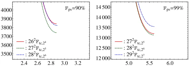
7.3 Optimal Number of Colors s
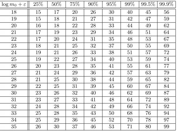
Let us plot the curves suggested in the previous subsection for some specific situations. Suppose that a certain set of parameters, achieving an intended suc-cess rate of Fps= 90% and appropriate for the resources available to a tradeoff implementer, is such that logm+ε= 26, whens= 24 is used. In the notation used in the previous subsection, this situation is expressed by logm0+ε= 22.
: 262Ftc,24 : 272Ftc,25 : 282Ftc,26
Fps=90%
2.4 2.6 2.8 3.0 3.2
3500 3600 3700 3800 3900 4000
: 272Ftc,25 : 282Ftc,26 : 292Ftc,27
Fps=99%
5.0 5.5 6.0
12 000 12 500 13 000 13 500 14 000 14 500
To find the optimal value ofsfor this situation, one must plot theFpc versus (22 + logs)2F
tc,s curves for varioussvalues. The left-hand side box of Figure 4
presents such curves for thesvalues of 24, 25, and 26, atF
ps = 90%. The switch from s= 24 to s= 25 moves the curve in the direction previously observed in Figure 3, but the transition froms= 25tos= 26results in a different behavior, that corresponds to a worsening of performance. The choice ofs= 25is seen to be optimal, at least among the powers of 2, for this situation.
The optimal choice ofscertainly would have been different if we had started from a different logm0+εvalue. The difference between the two boxes of Fig-ure 4 indicates that the optimal choice of s also depends on the success rate requirementFps.
We now wish to work with arbitrary integer values ofs and explicitly list the optimal value ofs, for a wide range of situations. The definition ofs being optimal must first be made clearer. It can be observed from the curves of Figure 4 that a curve that is generally lower than another curve has a lower lowest point. This vague claim cannot be written as a precise statement, since two curves may intersect each other and both be lower than the other at different parts of the curves. Nevertheless, the example curves of Figure 4 show that we would loose very little by choosing the curve or sto use, based on the lowest point of the curves. That is, for each choice of Fps and logm0+ε, we defining an s to be optimal, if it minimizes
min
Fmsc
n
{log(m0s) +ε}2Ftc,s
o
, (29)
i.e., the minimum value of the adjusted tradeoff coefficient.
Table 3 lists the optimal number of colorssto be used, for a small number of fixed success rate requirements Fps and a range of logm0+ε values. Since even the raw tradeoff coefficient Ftc,s does depend on s, theFmsc value giving the lowest point on each curve needs to be computed separately for eachs, but can still be obtained easily enough through numeric computations tools.
According to Table 3, the use of s = 31 is optimal for theFps = 90% and logm0+ε = 22 situation. Our previous suggestion to use s = 25, that was made after consulting the left-hand box of Figure 4, was quite reasonable. The table also statess = 48 to be optimal for theFps = 99% and logm0+ε = 22 situation. Our previous suggestion to uses= 26was somewhat large, but since 25 <48<26 and the curves for s= 25 ands = 26 in the right-hand side box of Figure 4 are very close to each other, this is not surprising and we are not experiencing any contradiction.
The overall observation we can make is that smallsvalues are optimal when under low success rate requirements and when the storage resources are small, and that largesvalues are optimal when working with the opposite environment.
8
Comparison of Tradeoff Algorithms
Table 3.The optimal number of colorssat various success probabilities and logm0+ε. logm0+ε 25% 50% 75% 90% 95% 99% 99.5% 99.9%
18 15 17 20 26 30 40 45 56
19 15 18 21 27 31 42 47 59
20 16 18 22 28 33 44 49 62
21 17 19 23 29 34 46 51 64
22 17 20 24 31 35 48 53 67
23 18 21 25 32 37 50 55 69
24 19 21 26 33 38 51 57 72
25 19 22 27 34 40 53 59 74
26 20 23 28 35 41 55 61 77
27 21 24 29 36 42 57 63 79
28 21 25 30 38 44 59 65 82
29 22 25 31 39 45 60 67 84
30 23 26 32 40 46 62 69 87
31 23 27 33 41 48 64 72 89
32 24 28 34 42 49 66 74 92
33 25 28 35 43 50 68 76 94
34 25 29 36 45 52 70 78 97
35 26 30 37 46 53 71 80 99
pre-computation coefficient versus tradeoff coefficient curves for the non-perfect fuzzy rainbow, perfect rainbow, and non-perfect rainbow tradeoffs at several fixed success rate requirements. Since the tradeoff coefficient is a good measure of the resources required during the online phase, the curves present the range of options made available by each algorithm concerning the degree of online efficiency that can be achieved after the investment of certain amount of pre-computation effort. The perfect and non-perfect rainbow tradeoffs were chosen as the comparison targets, because the two were shown by recent works [19, 20] to be the most competitive algorithms among the five major tradeoff algorithms, under typical conditions.
Instructions for plotting the Fpc versus Ftc,s curves for the fuzzy rainbow
tradeoff were given in Section 7.1, and the corresponding information for the comparison target algorithms can be found in [19, 20].
To compare the fuzzy rainbow tradeoff directly with the perfect and non-perfect rainbow tradeoffs, we need to find the appropriate adjustment factors to be multiplied to the tradeoff coefficients, and this starts with a discussion of the fuzzy rainbow tradeoff parameters mF, tF, ℓF, and s that would make the
resource requirements of the algorithm comparable to those of the perfect or non-perfect rainbow tradeoffs running under parametersmR,tR, andℓR.
We had mentioned in Remark 3 that the online time for the fuzzy rainbow tradeoff is of Θ(t2
Fs
2) order and we know that the online time for the usual rainbow tradeoff is of Θ(t2
R) order. Equating the very rough time and storage
ℓR≈1, we see that one must require
t2Fs
2
≈t2R and mFtF≈mFℓF≈mRℓR≈mR. (30)
These should be taken as extremely rough requirements, but the logarithm scale relations
logtF+ logs≈logtR and logmF+ logtF≈logmR (31)
are somewhat reasonably accurate requirements one should adhere to, if the two algorithms are to be using similar resources.
Recall from [19, 20] that each pre-computation table entry of both the perfect and non-perfect rainbow tradeoffs consumes logmR+εR bits of storage, where
εR is a small positive integer. We have already seen in Section 5 that the fuzzy
rainbow tradeoff similarly consumes logmF+εF bits of storage per table entry.
Our interest lies in the ratio of bits required per table entry, and the use of (31) implies
logmF+εF
logmR+εR ≈
logmR−logtR+ logs+εF
logmR+εR ≈
1
3logN+ logs+εF 2
3logN+εR
, (32)
where the second approximation is for the parameter setmR=N
2
3 andtR=N
1 3 that is typically considered during theoretical analyses of tradeoff algorithms. In the extreme, by ignoring the small integersεFandεR, and also assumingsto be
small, one might argue that this ratio could be as small as 1
2, at the theoretically typical parameters. However, this is a rather optimistic figure that is biased in favor of the fuzzy rainbow tradeoff.
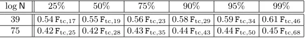
Let us briefly work with some specific numbers. The first example we consider is the very large search space of logN = 75, for which pre-computation could be barely within reach by very large organizations. We assumeεR≈εF≈8 bits
are used to record the ending point portions that remain after applications of the truncation and index file methods. When logN= 75, the rainbow tradeoff parameter set that is typically considered during theoretical treatments of the tradeoff technique is
logmR= 50 and logtR= 25. (33)
According to (31), the parameter set for the fuzzy rainbow tradeoff that calls for comparable resources would satisfy
logmF−logs≈logmR−logtR= 25. (34)
That is, we must take logm0 ≈ 25, in the notation of Section 7.2. The row labeled as logm0+εF= 33 in Table 3 states= 68 as the optimal choice, when
Fps= 99% is required. The ratio of bits per table entry is logmF+εF
logmR+εR ≈
25 + log 68 + 8
Table 4. The adjusted tradeoff coefficients for the fuzzy rainbow tradeoff that are appropriate for direct comparison against the usual rainbow tradeoff coefficients, as-suming the use of theoretically typical rainbow tradeoff parameters.
logN 25% 50% 75% 90% 95% 99%
39 0.54Ftc,17 0.55Ftc,19 0.56Ftc,23 0.58Ftc,29 0.59Ftc,34 0.61Ftc,46 75 0.42Ftc,25 0.42Ftc,28 0.43Ftc,35 0.44Ftc,43 0.44Ftc,50 0.45Ftc,68
Arguments similar to those made in Section 7.2 imply that, if one’s favored bal-ance of resources corresponds to rainbow tradeoff parameters of (33), one must compare the adjusted tradeoff coefficient 0.672F
tc,68 = 0.45Ftc,68 against the rainbow tradeoff coefficients Rtc (non-perfect) and ¯Rtc (perfect). Similar treat-ment of other success rates can be done, and the bottom row of Table 4 lists the adjusted tradeoff coefficients for the fuzzy rainbow tradeoff that would be appro-priate for comparisons againstRtcand ¯Rtc, when theoretically typical parameters for space size logN= 75 are considered.
The second example we consider is at the other extreme, and is the small search space size of logN = 39. Direct exhaustive search might even be rea-sonable for such small spaces. For this space size, the rainbow tradeoff param-eters logmR = 26 and logtR = 13 are theoretically typical, and if we assume
εR≈εF≈8, as in the previous example, we must accept
logm0+εF≈logmR−logtR+εR= 26−13 + 8 = 21. (36)
Table 3 shows that the use of s = 46 is optimal for the 99% success rate, in which case, the ratio of bits per table entry becomes
logmF+εF
logmR+εR ≈
13 + log 46 + 8
26 + 8 ≈0.780105. (37)
A fair comparison would let 0.782F
tc,46= 0.61Ftc,46compete againstRtcand ¯Rtc. Similar computations for other success rates can be done, and the outcomes are summarized in Table 4.
Different adjustment factors forFtc,s will need to be used, depending on the
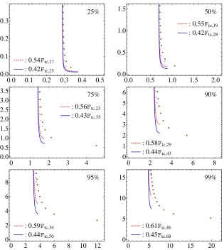
success rate requirement and rough range of online resources that are appro-priate for the situation in hand. However, we will somewhat arbitrarily choose to compare the two choices listed in Table 4, for each success rate, againstRtc and ¯Rtc. It seems reasonable to believe that our two choices represent the ex-treme situations that can be experienced during practical applications of the fuzzy rainbow tradeoff.
given above and to be given below can easily be adjusted to work for any specific situation. æ æ æ æ æ æ æ æ æ æ æ é é é é é é é é é é é
: 0.54Ftc,17
: 0.42Ftc,25
25%
0.0 0.1 0.2 0.3 0.4 0.5
0.0 0.1 0.2 0.3 æ æ æ æ æ æ æ æ æ æ é é é é é é é é é é
: 0.55Ftc,19
: 0.42Ftc,28
50%
0.0 0.5 1.0 1.5 2.0
0.0 0.5 1.0 1.5 æ æ æ æ æ æ æ æ é é é é é é
: 0.56Ftc,23
: 0.43Ftc,35
75%
0 1 2 3 4
0.0 0.5 1.0 1.5 2.0 2.5 3.0 3.5 æ æ æ æ æ æ æ é é é é
: 0.58Ftc,29
: 0.44Ftc,43
90%
0 2 4 6 8
0 1 2 3 4 5 6 æ æ æ æ æ æ æ æ æ é é é é é
: 0.59Ftc,34
: 0.44Ftc,50
95%
0 2 4 6 8 10 12
0 2 4 6 8 æ æ æ æ æ æ æ æ æ æ æ æ æ é é é é é
: 0.61Ftc,46
: 0.45Ftc,68
99%
0 5 10 15 20
0 5 10 15
Fig. 5. The rainbow tradeoff coefficients (Rtc: empty circles; ¯Rtc: filled dots) and the adjusted fuzzy rainbow tradeoff coefficients, in relation to their respective pre-computation costs, at various success rates (x-axis: pre-computation coefficient;y-axis: (adjusted) tradeoff coefficient).