An extended abstract of this paper is published in the proceedings of the 33rd Annual International Conference on the Theory and Applications of Cryptographic Techniques — Eurocrypt 2014. This is the full version.
Efficient Non-Malleable Codes and Key-Derivation
for Poly-Size Tampering Circuits
Sebastian Faust∗ Pratyay Mukherjee† Daniele Venturi‡ Daniel Wichs§
May 15, 2014
Abstract
Non-malleable codes, defined by Dziembowski, Pietrzak and Wichs (ICS ’10), provide roughly the following guarantee: if a codewordcencoding some messagexis tampered toc0=f(c) such thatc0 6=c, then the tampered messagex0contained inc0 reveals no information aboutx. Non-malleable codes have applications to immunizing cryptosystems against tampering attacks and related-key attacks.
Onecannothave anefficientnon-malleable code that protects againstall efficienttampering functions f. However, in this work we show “the next best thing”: for any polynomial bound s given a-priori, there is an efficient non-malleable code that protects against all tampering functions f computable by a circuit of size s. More generally, for any family of tampering functions F of size |F | ≤2s, there is an efficient non-malleable code that protects against all f ∈ F. Therateof our codes, defined as the ratio of message to codeword size, approaches 1. Our results are information-theoretic and our main proof technique relies on a careful probabilistic method argument using limited independence. As a result, we get an efficiently samplable family of efficient codes, such that a random member of the family is non-malleable with overwhelming probability. Alternatively, we can view the result as providing an efficient non-malleable code in the “common reference string” (CRS) model.
We also introduce a new notion of non-malleable key derivation, which uses randomness x to derive a secret key y =h(x) in such a way that, even if xis tampered to a different value x0 =f(x), the derived keyy0 =h(x0) does not reveal any information abouty. Our results for non-malleable key derivation are analogous to those for non-malleable codes.
As a useful tool in our analysis, we rely on the notion of “leakage-resilient storage” of Dav`ı, Dziembowski and Venturi (SCN ’10) and, as a result of independent interest, we also significantly improve on the parameters of such schemes.
∗
EPFL. Lausanne, Switzerland. E-mail: [email protected].
†
Aarhus University. Aarhus, Denmark. [email protected]. Research supported by a European Research Commission Starting Grant (no. 279447), the CTIC and CFEM research center.
‡
Sapienza University. Rome, Italy. E-mail: [email protected].
§
1
Introduction
Non-malleable codes were introduced by Dziembowski, Pietrzak and Wichs [20]. They provide meaningful guarantees on the integrity of an encoded message in the presence of tampering, even in settings where error-correction and error-detection may not be possible. Intuitively, a code (Enc,Dec) is non-malleable w.r.t. a family of tampering functionsF if the message contained in a codeword modified via a function f ∈ F is either the original message, or a completely unrelated value. For example, it should not be possible to just flip 1 bit of the message by tampering the codeword via a function f ∈ F. More formally, we consider an experiment Tamperfx in which a message x is (probabilistically) encoded to c ← Enc(x), the codeword is tampered to c0 = f(c) and, ifc0 6=c, the experiment outputs the tampered message x0 =Dec(c0), else it outputs a special value same?. We say that the code is non-malleable w.r.t. some family of tampering functions F
if, for every function f ∈ F and every messages x, the experiment Tamperfx reveals almost no information about x. More precisely, we say that the code is ε-non-malleable if for every pair of messages x, x0 and every f ∈ F, the distributions Tamperxf and Tamperfx0 are statistically ε-close.
The encoding/decoding functions are public and do not contain any secret keys. This makes the notion of non-malleable codes different from (but conceptually related to) the well-studied notions of non-malleability in cryptography, introduced by the seminal work of Dolev, Dwork and Naor [18]. Relation to Error Correction/Detection. Notice that non-malleability is a weaker guarantee than error correction/detection; the latter ensure that any change in the codeword can be corrected or at least detected by the decoding procedure, whereas the former does allow the message to be modified, but only to an unrelated value. However, when studying error correction/detection we usually restrict ourselves to limited forms of tampering which preserve some notion of distance (e.g., usually hamming distance) between the original and tampered codeword. (One exception is [14], which studies error-detection for more complex tampering.) For example, it is already impossible to achieve error correction/detection for the simple family of functionsFconst which, for every constant c∗, includes a “constant” function fc∗ that maps all inputs to c∗. There is always
some function in Fconst that maps everything to a valid codeword c∗. In contrast, it is trivial to construct codes that are non-malleable w.r.tFconst, as the output of a constant function is clearly independent of its input. The prior works on non-malleable codes, together with the results from this work, show that one can construct non-malleable codes for highly complex tampering function families F for which error correction/detection are unachievable.
Applications to Tamper Resilience. The fact that non-malleable codes can be built for large and complex families of functions makes them particularly attractive as a mechanism for protecting memory against tampering attacks, known to be a serious threat for the security of cryptographic schemes [8, 2, 30, 13]. As shown in [20], to protect a scheme with some secret state against memory-tampering, we simply encode the state via a non-malleable code and store the encoding in the memory instead of the original secret. One can show that if the code is non-malleable with respect to function family F, the transformed system is secure against tampering attacks carried out by any function in F. See [20] for a discussion of the application of non-malleable codes to tamper resilience.
Limitations & Possibility. It isimpossible to have codes that are non-malleable forall possible tampering functions. For any coding scheme (Enc,Dec), there exists a tampering function fbad(c)
c0 of x0. Notice that ifEnc,Dec are efficient, then the function fbad is efficient as well. Thus, it is
also impossible to have anefficient code which is non-malleable w.r.t all efficient functions. Prior works [27, 11, 19, 1, 10, 21] (discussed shortly) constructed non-malleable codes for several rich and interesting function families. In all cases, the families are restricted through theirgranularityrather than their computationalcomplexity. In particular, these works envision that the codeword is split into several (possibly just 2) components, each of which can only be tampered independently of the others. The tampering function therefore only operates on a “granular” rather than “global” view of the codeword.
1.1 Our Contribution
In this work, we are interested in designing non-malleable codes for large families of functions which are only restricted by their “computational complexity” rather than “granularity”. As we saw, we cannot have a single efficient code that is non-malleable for all efficient tampering functions. However, we show the following positive result, which we view as the “next best thing”:
Main Result: For any polynomial bound s = s(n) in the codeword size n, and any tampering family F of size |F | ≤ 2s, there is an efficient code of complexity poly(s,log(1/ε)) which is
ε-non-malleable w.r.t. F. In particular, F can be the family of all circuits of size at most s. The code is secure in the information theoretic setting, and achievesoptimal rate(message/codeword size) arbitrarily close to 1. It has asimple construction relying only ont-wise independent hashing. The CRS Model. In more detail, if we fix some familyF of tampering functions (e.g., circuits of bounded size), our result gives us a family of efficient codes, such that, with overwhelming probability, a random member of the family is non-malleable w.r.t F. Each code in the family is indexed by some hash functionhfrom at-wise independent family of hash functionsH. This result already shows the existence of efficient non-malleable codes with some small non-uniform advice to indicate a “good” hash functionh.
However, we can also efficiently sample a random member of the code family by sampling a random hash functionh. Therefore, we find it most appealing to think of this result as providing a uniformly efficient construction of non-malleable codes in the “common reference string (CRS)” model, where a random public string consisting of the hash function h is selected once and fixes the non-malleable code. We emphasize that, although the familyF (e.g., circuits of bounded size) is fixed prior to the choice of the CRS, the attacker can choose the tampering functionf ∈ F (e.g., a particular small circuit) adaptively depending on the choice of h.
We argue that it is unlikely that we can completely de-randomize our construction and come up with a fixed uniformly-efficient code which is non-malleable for all circuits of size (say)s=O(n2). In particular, this would require a circuit lower bound, showing that the function fbad (described
above) cannot be computed by a circuit of size O(n2).
While we believe that non-malleable key derivation is an interesting notion on its own (e.g., it can be viewed as a dual version of non-malleable extractors [17]), we also show it has useful applications for tamper resilience. For instance, consider some cryptographic scheme G using a uniform key in y ← {0,1}k. To protect G against tampering attacks, we can store a bigger key
x ← {0,1}n on the device and temporarily derive y =h(x) each time we want to execute G. In Appendix A, we show that this approach protects any cryptographic scheme with a uniform key against one-time tampering attacks. The main advantage of using a non-malleable key-derivation rather than non-malleable codes is that the keyx stored in memory is simply a uniformly random string with no particular structure (in contrast, the codeword in a non-malleable code requires structure).
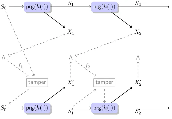
In Section 6, we also show how to use non-malleable key derivation to build a tamper-resilient stream cipher. Our construction is based on a PRGprg:{0,1}k → {0,1}n+v and a non-malleable key derivation function h :{0,1}n → {0,1}k. For an initial key s0 ← {0,1}n, sampled uniformly at random, the output of the stream cipher at each roundi∈[q] is (si, xi) :=prg(h(si−1)).
1.2 Our Techniques
Non-Malleable Codes. Our construction of non-malleable codes is incredibly simple and relies ont-wise independent hashing, wheretis proportional tos= log|F |. In particular, ifh1, h2are two such hash functions, we encode a message x into a codeword c= (r, z, σ) where r is randomness,
z=x⊕h1(r) andσ=h2(r, z). The security analysis, on the other hand, requires two independently interesting components. Firstly, we rely on the notion of leakage-resilient encodings, proposed by Dav`ı, Dziembowski and Venturi [16]. These provide a method to encode a secret in such a way that a limited form of leakage on the encoding does not reveal anything about the secret. One of our contributions is to significantly improve the parameters of the construction from [16] by using a fresh and more careful analysis, which gives us such schemes with an essentially optimal rate. Secondly, we analyze a simpler/weaker notion ofbounded non-malleability, which intuitively guarantees that an adversary seeing the decoding of a tampered codeword can learn only a bounded amount of information on the encoded value. This notion of bounded non-malleability is significantly simpler to analyze than full non-malleability. Finally, we show how to carefully combine leakage-resilient encodings with bounded non-malleability to get our full construction of non-malleable codes. On a very high (and not entirely precise) level, we can think ofh1above as providing “leakage resilience” and h2 as providing “bounded non-malleability”.
We stress that the fact thatthas to be proportional tosis not an artefact of our proof. In fact, one can see that whenever the hash function has seed size s, there is a family of 2s functions that breaks the construction with probability 1: For each seed, just have a new function that decodes with that seed and encodes a related value. This shows that thethas to be proportional to log|F |. Non-Malleable Key-Derivation. Our construction of non-malleable key-derivation functions is even simpler: a randomt-wise independent hash function h already satisfies the definition with overwhelming probability, wheret is proportional tos= log|F |. The analysis is again subtle and relies on a careful probabilistic method argument.
Similar to the case of non-malleable codes, the fact thatthas to be proportional tosis necessary.
1.3 Related Works
codeword independently. The original work of [20] (see also [12]) gives an efficient construction for bit-tampering (i.e., the adversary can tamper with each bit of the codeword independently of every other bit). Very recently, Cheraghchi and Guruswami [10] gave a construction with improved rate and better efficiency for the same family. Choiet al.[11] considered an extended tampering family, where the tampering function can be applied to a small (logarithmic in the security parameter) number of blocks independently.
Perhaps the least granular and most general such model is the so-calledsplit-state model, where the encoding consists of two parts L (left) and R (right), and the adversary can tamper L and R
arbitrarily but independently. Starting with the random oracle construction of [20], a few other constructions of non-malleable split-state codes have been proposed, both in the computational setting [27, 21] and in the information theoretic setting [19, 1, 10]. Notice that the family Fsplit
of all split-state tampering functions (without restricting efficiency), has doubly exponential size 2O(2n/2) in the codeword size n, and therefore it is not covered by our results, which can efficiently handle at most singly-exponential-size families 2poly(n). On the other hand, the split-state model doesn’t cover “computationally simple” functions, such as the function computing the XOR or the bit-wise inner-product ofL, R. Therefore, although the works are technically orthogonal, we believe that looking at computational complexity may be more natural.
Global Tampering. The work of [20] gives an existential (inefficient) construction of non-malleable codes for doubly-exponential sized function families. More precisely, for any constant 0 < α < 1 and any family F of functions of size |F | ≤ 22αn in the codeword size n, there exists an inefficient non-malleable code w.r.t.F; indeed a completely random function gives such a code with high probability. The code is clearly not efficient, and this should be expected for such a broad result: the familiesF can include all circuits of size (e.g.,)s(n) = 2n/2, which means that the efficiency of the code must exceedO(2n/2). Unfortunately, there is no direct way to “scale down” the result in [20] so as to get an efficient construction for singly-exponential-size families. (One can view our work as providing such “scaled down” result.) Moreover, the analysis only yielded a rate of at most (1−α)/3<1/3, and it was previously not known if such codes can achieve a rate close to 1, even for “small” function families. We note that [20] also showed that the probabilistic method construction can yield efficient non-malleable codes for large function families in therandom oracle model. However, this only considers function families that don’t have access to the random oracle. For example, one cannot interpret this as giving any meaningful result for tampering functions with bounded complexity.
Concurrent and Independent Work. In a concurrent and independent work, Cheraghchi and Guruswami [9] give two related results. Firstly, they improve the probabilistic method construc-tion of [20] and show that, for families F of size |F | ≤ 22αn, there exist (inherently inefficient) non-malleable codes with rate 1−α, which they also show to be optimal. This gives the first char-acterization of the rate of non-malleable codes. Secondly, similar to our results, they use limited independence to construct efficient non-malleable codes when restricted to tampering families F
Other Approaches to Achieve Tamper Resilience. There is a vast body of literature that considers tampering attacks using other approaches besides non-malleable codes. See, e.g., [5, 23, 25, 4, 22, 26, 3, 24, 28, 31, 6, 15]. The reader is referred to (e.g.,) [20] for a more detailed comparison between these approaches and non-malleable codes.
2
Preliminaries
Notation. We denote the set of first n natural numbers, i.e. {1, . . . , n}, by [n]. Let X, Y be random variables with supportsS(X), S(Y), respectively. We define
SD(X, Y)def= 1 2
X
s∈S(X)∪S(Y)
|Pr[X =s]−Pr[Y =s]|
to be theirstatistical distance. We write X≈εY and say thatX and Y are ε-statistically close to
denote that SD(X, Y) ≤ε. We let Un denote the uniform distribution over {0,1}n. We use the
notation x←X to denote the process of sampling a valuex according to the distributionX. Iff
is a randomized algorithm, we writef(x;r) to denote the execution off on input x with random coinsr. We letf(x) denote a random variable over the random coins.
We recall two lemmas from [7].
Lemma 2.1 (Lemma 2.3 of [7]). Let t ≥ 4 be an even integer. Suppose X1, . . . , Xn are t-wise
independent random variables taking values in [0,1]. Let X := Pn
i=1Xi and define µ:= E[X] be
the expectation of the sum. Then, for any A >0, Pr[|X−µ| ≥A]≤Kt
tµ+t2
A2 t/2
where Kt≤8.
Lemma 2.2 (Lemma A.1 of [7]). Let t≥2 be an even integer. Suppose X1, X2, . . . , Xn are t-wise
independent random variables taking values in [0,1]. Let X := Pn
i=1Xi and µ := E[X] be the
expectation of the sum. Then, E[(X−µ)t]≤K
t tµ+t2
t/2
where Kt≤8.
Notice that Lemma 2.2 is slightly modified from Lemma A.1 of [7], where the random variables are fully independent. However it is easy to extend the statement in [7] to the one above by a simple observation (also stated in [7]) that, by linearity of expectation, the value of E[(X−µ)t] can be computed under the assumption that X1, . . . , Xn are fully independent, whenever they are
at leastt-wise independent.
2.1 Definitions of Non-Malleable Codes
Definition 2.3 (Coding Scheme). A(k, n)-coding scheme consists of two functions: a randomized encoding function Enc :{0,1}k → {0,1}n, and a deterministic decoding function Dec :{0,1}n → {0,1}k∪ {⊥} such that, for eachx∈ {0,1}k, Pr[Dec(Enc(x)) =x] = 1.
Definition 2.4 (Strong Non-Malleability [20]). Let (Enc,Dec) be a (k, n)-coding scheme and F be a family of functionsf : {0,1}n→ {0,1}n. We say that the scheme is (F, ε)-non-malleable if for anyx0, x1 ∈ {0,1}k and any f ∈ F, we have Tamperfx0 ≈εTamper
f
x1 where
Tamperfxdef=
c←Enc(x), c0 :=f(c), x0=Dec(c0) Output same? if c0=c, andx0 otherwise.
.
For super non-malleable security (defined below), if the tampering manages to modify c to c0
such thatc0 6=c andDec(c0)6=⊥, then we will even give the attacker the tampered codeword c0 in full rather than just givingx0 =Dec(c0). We do not immediately see a concrete application of this strengthening, but it seems sufficiently interesting to define explicitly.
Definition 2.5 (Super Non-Malleability). Let (Enc,Dec) be a (k, n)-coding scheme and F be a family of functions f : {0,1}n → {0,1}n. We say that the scheme is (F, ε)-super non-malleable if for anyx0, x1 ∈ {0,1}k and any f ∈ F, we have Tamperfx0 ≈εTamper
f
x1 where:
Tamperfx def=
c←Enc(x), c0 :=f(c)
Output same? if c0 =c, output ⊥if Dec(c0) =⊥,
and else outputc0.
.
3
Improved Leakage-Resilient Codes
We will rely on leakage resilience as an important tool in our analysis. The following notion of leakage-resilient codes was defined by [16]. Informally, a code is leakage-resilient w.r.t. some leakage familyF if, for any f ∈ F, “leaking”f(c) for a codewordcdoes not reveal anything about the encoded value.
Definition 3.1(Leakage-Resilient Codes [16]). Let(LREnc,LRDec) be a(k, n)-coding scheme. For a function family F, we say that (LREnc,LRDec) is (F, ε)-leakage-resilient, if for any f ∈ F and anyx∈ {0,1}k we have SD(f(LREnc(x)), f(Un))≤ε.
The work of [16] gave a probabilistic method construction showing that such codes exist and can be efficient when the size of the leakage family |F | is singly-exponential. However, the rate
k/n was at most some small constant (< 14), even when the family size |F | and the leakage size
` are small. Here, we take the construction of [16] and give an improved analysis with improved parameters, showing that the rate can approach 1. In particular, the additive overhead of the code is very close to the leakage-amount `, which is optimal. Our result and analysis are also related to the “high-moment crooked leftover hash lemma” of [29], although our construction is somewhat different, relying only on high-independence hash functions rather than permutations.
Construction. LetHbe at-wise independent function family consisting of functionsh : {0,1}v → {0,1}k. For any h ∈ H we define the (k, n = k+v)-coding scheme (LREnch,LRDech) where: (i)
LREnch(x) := (r, h(r)⊕x) for r ← {0,1}v; (ii)LRDech((r, z)) :=z⊕h(r).
Theorem 3.2. Fix any function family F consisting of functions f : {0,1}n → {0,1}`. With probability 1−ρ over the choice of a random h ← H, the coding scheme (LREnch,LRDech) is
(F, ε)-leakage-resilient as long as:
Proof. Fix a function family F. Now, taking probabilities (only) over the choice of h, let Badbe
the event that (LREnc,LRDec) is not an (F, ε)-leakage-resilient code. Then, Pr[Bad] = Pr
h←H[∃f ∈ F, x∈ {0,1}
k : SD(f(LREnc
h(x)), f(Un))> ε]
≤ X
f∈F X
x∈{0,1}k Pr
h←H
X
α∈{0,1}`
Pr
r←{0,1}v[f(r, h(r)
⊕x) =α]−Pr[f(Un) =α]
>2ε
(1)
where Eq. (1) follows by taking a union bound over all f ∈ F and x∈ {0,1}k.
Fix any f ∈ F, x ∈ {0,1}k. For any α ∈ {0,1}`, r ∈ {0,1}v, define pα := Pr[f(Un) = α] and
pr,α := Pr[f(r, Uk) =α]. Let peα := max{ pα , 2
−` }. Note that
X
α∈{0,1}` e
pα≤
X
α
pα+
X
α
2−` ≤2. (2)
Define the random variable Yr,α such that Yr,α = 1 if f(r, h(r)⊕x) = α, where the randomness
is over the choice of h ← H. Then Pr[Yr,α = 1] = pr,α and, for a fixed α, the random variables
{Yr,α}r∈{0,1}v aret-wise independent. Moreover, E[P
r∈{0,1}vYr,α] = 2vpα. Therefore, we have:
Pr
h←H
X
α∈{0,1}`
Pr
r←{0,1}v[f(r, h(r)⊕x) =α]−Pr[f(Un) =α]
>2ε
≤ Pr
h←H
∃α∈ {0,1}` :
Pr
r←{0,1}v[f(r, h(r)⊕x) =α]−pα
> ε·peα
(3)
≤ X
α∈{0,1}` Pr h←H X
r∈{0,1}v
Yr,α−2vpα
>2vε·peα
≤ X
α∈{0,1}`
Kt
t2vpα+t2
(2vε
e
pα)2
t/2
(4)
≤ X
α∈{0,1}`
Kt
2t2v·peα
(2vε
e
pα)2
t/2
≤2`Kt
2t
2v−`ε2 t/2
, (5)
where (3) follows from (2), and (4) follows from Lemma 2.1, withKt≤8. Finally, (5) follow from
the fact that the theorem’s parameters ensure: 2v·peα≥2v−`≥t.
Combining the above with (1), we get: Pr[Bad]≤ |F | ·2`+k·8 2v−2t`ε2 t/2
. Therefore to satisfy Pr[Bad]≤ρ we can set:
v≥`+ 2 log(1/ε) + log(t) + 3 and t≥log|F |+`+k+ log(1/ρ) + 3.
4
Non-Malleable Codes
Construction. LetH1 be a family of hash functionsh1 : {0,1}v1 → {0,1}k, andH2 be a family of hash functionsh2 : {0,1}k+v1 → {0,1}v2 such thatH1 andH2are botht-wise independent. For any (h1, h2)∈ H1× H2, define Ench1,h2(x) = (r, z, σ) wherer ← {0,1}
v1 is random,z:=x⊕h 1(r) and σ :=h2(r, z). The codewords are of size n:=|(r, z, σ)|=k+v1+v2. Correspondingly define
Dec((r, z, σ)) which first checksσ =? h2(r, z) and if this fails, outputs⊥, else outputsz⊕h1(r). Notice that, we can think of (r, z) as being a leakage-resilient encoding ofx; i.e., (r, z) =LREnch1(x;r). Theorem 4.1. For any function family F, the above construction (Ench1,h2,Dech1,h2)is an (F, ε )-super non-malleable code with probability 1−ρ over the choice of h1, h2 as long as:
t≥t∗ for some t∗ =O(log|F |+n+ log(1/ρ))
v1 > v∗1 for some v ∗
1 = 3 log(1/ε) + 3 log(t ∗
) +O(1)
v2 > v1+ 3.
For example, in the above theorem, if we set ρ = ε = 2−λ for “security parameter” λ, and
|F | = 2s(n) for some polynomial s(n) = nO(1) ≥ n ≥ λ, then we can set t = O(s(n)) and the message length k := n−(v1 +v2) = n−O(λ+ logn). Therefore the rate of the code k/n is 1−O(λ+ logn)/n which approaches 1 asn grows relative toλ.
4.1 Proof of Theorem 4.1
Useful Notions. For a coding scheme (Enc,Dec), we say thatc∈ {0,1}n isvalid ifDec(c)6=⊥. For any functionf : {0,1}n→ {0,1}n, we say thatc0 ∈ {0,1}n isδ-heavy forf if Pr[f(Enc(Uk)) =
c0]≥δ. Define
Hf(δ) ={c0∈ {0,1}n : c0 isδ-heavy forf}.
Notice that |Hf(δ)| ≤1/δ.
Definition 4.2(Bounded-malleable). We say that a coding scheme(Enc,Dec)is(F, δ, τ )-bounded-malleable if for all f ∈ F, x∈ {0,1}k we have
Pr[c0 6=c∧c0 is valid ∧c0 6∈Hf(δ) | c←Enc(x), c0 =f(c)]≤τ,
where the probability is over the randomness of the encoding.
Intuition. The above definition says the following. Take any message x ∈ {0,1}k, tampering function f ∈ F and do the following: choose c ← Enc(x), set c0 = f(c), and output: (i) same? if
c0 = c, (ii) ⊥ if c0 is not valid, (iii) c0 otherwise. Then, with probability 1−τ the output of the above experiment takes on one of the values: {same?,⊥} ∪Hf(δ). Therefore, the output of the
From Bounded-Malleable to Non-Malleable. For any “tampering function” family F con-sisting of functionsf : {0,1}n→ {0,1}n, anyδ >0, and anyh2 ∈ H2 we define the “leakage func-tion” familyG =G(F, h2, δ) which consists of the functions gf : {0,1}k+v1 →Hf(δ)∪ {same?,⊥}
for each f ∈ F. The functions are defined as follows:
• gf(c1): Compute σ =h2(c1). Let c := (c1, σ), c0 = f(c). If c0 is not valid output ⊥. Else if
c0 = c output same?. Else if c0 ∈ Hf(δ) output c0. Lastly, if none of the above cases holds,
output ⊥.
Notice that the notion of “δ-heavy” and the set Hf(δ) are completely specified by h2 and do not depend on h1. This is because the distribution Ench1,h2(Uk) is equivalent to (Uk+v1, h2(Uk+v1)) and therefore c0 is δ-heavy if and only if Pr[f(Uk+v1, h2(Uk+v1)) = c
0]≥ δ. Therefore the family G=G(F, h2, δ) is fully specified byF, h2, δ. Also notice that|G|=|F | and that the output length of the functionsgf is given by `=dlog(|Hf(δ)|+ 2)e ≤ dlog(1/δ+ 2)e.
Lemma 4.3. LetF be any function family and letδ >0. Fix anyh1, h2such that(Ench1,h2,Dech1,h2) is(F, δ, ε/4)-bounded-malleable and(LREnch1,LRDech1)is(G(F, h2, δ), ε/4)-leakage-resilient, where the family G = G(F, h2, δ), with size |G| = |F |, is defined above, and the leakage amount is
`=dlog(1/δ+ 2)e. Then (Ench1,h2,Dech1,h2) is (F, ε)-non-malleable. Proof. For any x0, x1∈ {0,1}k and any f ∈ F:
Tamperfx0 =
c←Ench1,h2(x0), c
0:=f(c) Output: same? ifc0=c,⊥ifDech1,h2(c
0) =⊥,
c0 otherwise.
stat ≈ε/4
c1 ←LREnch1(x0) Output: gf(c1)
(6) stat
≈ε/4
c1 ←LREnch1(Uk) Output: gf(c1)
(7) stat
≈ε/4
c1 ←LREnch1(x1) Output: gf(c1)
(8)
stat ≈ε/4
c←Ench1,h2(x1), c
0:=f(c) Output: same? ifc0=c,⊥ifDec
h1,h2(c
0) =⊥,
c0 otherwise.
(9)
=Tamperfx1.
Eq. (6) and Eq. (9) follow as (Ench1,h2,Dech1,h2) is an (F, δ, ε/4)-bounded-malleable code, and Eq. (7) and Eq. (8) follow as the code (LREnch1,LRDech1) is (G(F, δ), ε/4)-leakage-resilient.
We can use Theorem 3.2 to show that (LREnch1,LRDech1) is (G(F, h2, δ), ε/4)-leakage-resilient with overwhelming probability. Therefore, it remains to show that our construction is (F, δ, τ )-bounded-malleable, which we do below.
following two properties hold for any messagexand any functionf with overwhelming probability: (i) there is at most some “small” set of q valid codewords c0 that we can hit by tampering some encoding of x via f; (ii) for each such codeword c0 which is not in δ-heavy, the probability of landing inc0 after tampering an encoding ofxcannot be higher than 2δ. This shows that the total probability of tampering an encoding ofxand landing in a valid codeword which not δ-heavy is at most 2qδ, which is small. Property (i) roughly follows by showing that f would need to “predict” the output of h2 onq different inputs, and property (ii) follows by using “leakage resilience” ofh1 to argue that we cannot distinguish an encoding ofx from an encoding of a random message, for which the probability of landing in c0 is at most δ.
Lemma 4.4. For any function family F, any δ > 0, the code (Ench1,h2,Dech1,h2) is (F, δ, τ )-bounded-malleable with probability 1−ψ over the choice of h1, h2 as long as:
τ ≥ 2(log|F |+k+ log(1/ψ) + 2)δ t ≥ log|F |+n+k+ log(1/ψ) + 5
v1 ≥ 2 log(1/δ) + log(t) + 4 and v2≥v1+ 3.
Proof. Setq :=dlog|F |+k+ log(1/ψ) + 1e. For any f ∈ F, x∈ {0,1}k define the eventsE1f,x and
E2f,x over the random choice ofh1, h2 as follows:
1. E1f,x occurs if there exist at least q distinct values c01, . . . , cq0 ∈ {0,1}n such that each c0i is valid and c0i = f(ci) for some ci 6=c0i which encodes the message x (i.e., ci =Ench1,h2(x;ri) for someri).
2. E2f,x occurs if there exists somec0∈ {0,1}n\Hf(δ) such that Prr←{0,1}v1[f(Ench1,h2(x;r)) =
c0]≥2δ.
LetE1 =Wf,xE1f,x, E2 =Wf,xE2f,x and Bad=E1∨E2. Assume (h1, h2) are any hash functions for which the eventBad doesnot occur. Then, for every f ∈ F, x∈ {0,1}k:
Pr[f(C)6=C∧f(C) is valid ∧f(C)6∈Hf(δ)]
= X
c0:c0valid andc06∈H
f(δ)
Pr[f(C) =c0∧C =6 c0]<2qδ≤τ, (10)
where C = Ench1,h2(x;Uv1) is a random variable. Eq. (10) holds since (i) given that E1 does not occur, there are fewer than q values c0 that are valid and for which Pr[f(C) = c0∧C 6=c0]> 0, and (ii) given that E2 does not occur, for any c0 6∈Hf(δ), we also have Pr[f(C) =c0 ∧C 6=c0]≤
Pr[f(C) =c0]<2δ.
Therefore, if the event Baddoes not occur, then the code is (F, δ, τ)-bounded-malleable. This
means: Pr
h1,h2
[(Ench1,h2,Dech1,h2) is not (F, δ, τ)-bounded-malleable]≤Pr[Bad]≤Pr[E1] + Pr[E2]. So it suffices to show that Pr[E1] and Pr[E2] are both bounded by ψ/2, which we do next.
Claim 4.5. Pr[E1]≤ψ/2.
Proof. Fix some messagex∈ {0,1}k and some functionf ∈ F. Assume that the eventE1f,x occurs for some choice of hash functions (h1, h2). Then there must exist some values {r1, . . . , rq} such
last condition also implies |{c1, . . . , cq}|= q. However, it is possible that ci = c0j for some i6= j.
We claim that we can find a subset of at least s := dq/3e of the indices such that the 2s values
{ca1, . . . , cas, c 0
a1, . . . , c 0
as} are all distinct. To do so, notice that if we want to keep some index i
corresponding to valuesci, c0i, we need to take out at most two indicesj,kin casecj0 =ciorck=c0i.1
To summarize, if E1f,x occurs, then (by re-indexing) there is some setR ={r1, . . . , rs} ⊆ {0,1}v1
of size |R|=ssatisfying the following two conditions:
(i) If we define ci := Enc(x;ri), c0i 6= ci and ci0 is valid meaning that c0i = (ri0, zi0, σi0) where
σ0 =h2(r0, z0).
(ii) |{c1, . . . , cs, c01, . . . , c0s}|= 2s.
Therefore we have: Pr[E1f,x] ≤ Pr
h1,h2
[∃R⊆ {0,1}v1,|R|=s, R satisfies (i) and (ii)]≤X
R
Pr
h1,h2
[R satisfies (i) and (ii)]
≤ X
R={r1,...,rs}
max
h1,σ1,...,σs
Pr
h2
∀i , c0i valid
ci := (ri, zi =h1(ri)⊕x, σi), c0i:=f(ci), c0i 6=ci
|{c1, . . . , cs, c01, . . . , c0s}|= 2s
≤
2v1
s
2−sv2 ≤
e2v1
s
s
2−sv2 ≤2s(v1−v2) ≤2q(v1−v2)/3 ≤2−q, (11) where Eq. (11) follows from the fact that, even if we condition on any choice of the hash function
h1 which fixes zi = h1(ri)⊕x, and any choice of the s values σi = h2(ri, zi), which fixes ci :=
(ri, zi = h1(ri)⊕x, σi), c0i := f(ci) such that c0i 6= ci and |{c1, . . . , cs, c01, . . . , c0s}| = 2s, then the
probability thath2(r0i, z
0
i) =σ
0
i for alli∈[s] is at most 2
−sv2. Here we use the fact thatH
2 ist-wise independent wheret≥q≥2s. Now, we calculate
Pr[E1]≤ X
f∈F X
x∈{0,1}k
Pr[Ef,x1 ]≤ |F |2k−q ≤ψ/2,
where the last inequality follows from the assumption,q =dlog|F |+k+ log(1/ψ) + 1e. Claim 4.6. Pr[E2]≤ψ/2.
Proof. For this proof, we will rely on the leakage resilience property of the code (LREnch1,LRDech1) as shown in Theorem 3.2. First, let us write:
Pr[E2] = Pr
h1,h2 h
∃(f, x, c0)∈ F × {0,1}k× {0,1}n\Hf(δ) : Pr[f(Ench1,h2(x;Uv1)) =c 0
]≥2δ
i
≤ Pr
h1,h2
∃(f, x, c0)∈ F × {0,1}k× {0,1}n\Hf(δ) : (12)
Pr[f(Ench1,h2(x;Uv1)) =c0]−Pr[f(Ench1,h2(Uk;Uv1)) =c0] ≥δ
since, for any c0 6∈Hf(δ), we have Pr[f(Ench1,h2(Uk;Uv1)) =c
0]< δ by definition. Notice that we can write Ench1,h2(x;r) = (c1, c2) where c1 =LREnch1(x;r), c2 =h2(c1). We will now rely on the leakage resilience of the code (LREnch1,LRDech1) to bound the above probability by ψ/2. In fact,
1
In other words, if we take any set of tuples{(ci, c0i)}such that all the left components are distinctci6=cj and
all the right components are distinctc0i6=c
0
j, but there may be common valuesci =c0j, then there is a subset of at
we show that the above holds even if we take the probability over h1 only, for a worst-case choice of h2.
Let us fix some choice of h2 and define the family G = G(h2) of leakage functions G = {gf,c0 : {0,1}k+v1 → {0,1} | f ∈ F, c0 ∈ {0,1}n} with output size `= 1 bits as follows:
• gf,c0(c1): Setc= (c1, c2 =h2(c1)). If f(c) =c0 output 1, else output 0.
Notice that the size of the family G is 2n|F | and the family does not depend on the choice of h1. Therefore, continuing from inequality (12), we get:
Pr[E2] ≤ Pr
h1,h2
∃(f, x, c0)∈ F × {0,1}k× {0,1}n\Hf(δ) :
Pr[f(Ench1,h2(x;Uv1)) =c0]−Pr[f(Ench1,h2(Uk;Uv1)) =c0] ≥δ
≤ max
h2 Pr
h1
∃(gf,c0, x)∈ G(h2)× {0,1}k :
Pr[gf,c0(LREnch
1(x;Uv1)) = 1]
−Pr[gf,c0(LREnch
1(Uk;Uv1)) = 1]
≥δ
= max
h2 Pr
h1
∃(gf,c0, x)∈ G(h2)× {0,1}k :
Pr[gf,c0(LREnch
1(x;Uv1)) = 1]
−Pr[gf,c0(Uk+v
1) = 1]
≥δ
≤ max
h2 Pr
h1
[ (LREnch1,LRDech1) is not (G(h2), δ)-Leakage-Resilient ]≤ψ/2,
where the last inequality follows from Theorem 3.2 by the choice of parameters.
Putting it All Together. Lemma 4.3 tells us that for any δ >0 and any function family F: Pr[(Ench1,h2,Dech1,h2) is not (F, ε)-super-non-malleable]
≤Pr[(Ench1,h2,Dech1,h2) is not (F, δ, ε/4)-bounded-malleable] (13) + Pr[(LREnch1,LRDech1) is not (G(F, h2, δ), ε/4)-leakage-resilient], (14) whereG =G(F, h2, δ) is of size|G|=|F |and consists of function with output size`=dlog(1/δ+2)e. Let us set δ := (ε/8)(log|F |+k+ log(1/ρ) + 3)−1. This ensures that the first requirement of Lemma 4.4 is satisfied with τ = ε/4. We choose t∗ = O(log|F | +n+ log(1/ρ)) such that log(1/δ)≤log(1/ε) + log(t∗) +O(1). Notice that the leakage amount of G is `=dlog(1/δ+ 2)e ≤
log(1/ε) + log(t∗) +O(1). With v1, v2 as in Theorem 4.1, we satisfy the remaining requirements of Lemma 4.4 (bounded-malleable codes) and Theorem 3.2 (leakage-resilient codes) to ensure that the probabilities (13), (14) are both bounded byρ/2, which proves our theorem.
5
Non-Malleable Key-Derivation
In this section we introduce a new primitive, which we name non-malleable key derivation. Intu-itively a functionhis a non-malleable key derivation function ifh(x) is close to uniform even given the output ofh applied to a related inputf(x), as long asf(x)6=x.
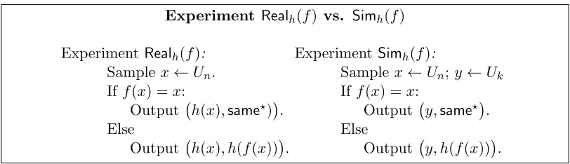
Definition 5.1 (Non-Malleable Key-Derivation). Let F be any family of functionsf : {0,1}n→ {0,1}n. We say that a function h : {0,1}n → {0,1}k is an (F, ε)-non-malleable key derivation function if for every f ∈ F we have SD Realh(f); Simh(f)
≤ ε where Realh(f) and Simh(f)
Experiment Realh(f) vs. Simh(f)
Experiment Realh(f):
Samplex←Un.
Iff(x) =x:
Output h(x),same?) . Else
Output h(x), h(f(x)).
Experiment Simh(f):
Sample x←Un;y←Uk
If f(x) =x:
Output y,same? . Else
Output y, h(f(x)).
Figure 1: Experiments defining a non-malleable key derivation functionh
Note that the above definition can be interpreted as a dual version of the definition of non-malleable extractors [17].2 The theorem below states that by sampling a function h from a set
H of t-wise independent hash functions, we obtain a non-malleable key derivation function with overwhelming probability.
Theorem 5.2. LetHbe a2t-wise independent function family consisting of functionsh : {0,1}n→ {0,1}k and letF be some function family as above. Then with probability1−ρ over the choice of a random h← H, the functionh is an (F, ε)-non-malleable key-derivation function as long as:
n≥2k+ log(1/ε) + log(t) + 3 and t >log(|F |) + 2k+ log(1/ρ) + 5.
Proof. For any h ∈ H and f ∈ F, define a function hf : {0,1}n → {0,1}k∪same? such that if
f(x) = x then hf(x) = same? otherwise hf(x) = h(f(x)). Fix a function family F. Now, taking
probabilities (only) over the choice ofh, letBadbe the event thathis not an (F, ε
)-non-malleable-key-derivation function. Then: Pr[Bad] = Pr
h←H
∃f ∈ F : SD( Realh(f) , Simh(f) )> ε
= Pr
h←H
∃f ∈ F : SD( (h(X), hf(X)), (Uk, hf(X)) )> ε
≤ X f∈F Pr h←H X
y∈{0,1}k
X
y0∈{0,1}k∪same?
Pr[h(X) =y∧hf(X) =y0]
−Pr[Uk =y∧hf(X) =y0]
>2ε
≤ X f∈F Pr h←H
∃ y∈ {0,1}k, y0 ∈ {0,1}k∪same? :
Pr[h(X) =y∧hf(X) =y0]
−Pr[Uk=y∧hf(X) =y0]
>2−2kε
≤ X
f∈F X
y∈{0,1}k
X
y0∈{0,1}k∪ same? Pr h←H
Pr[h(X) =y∧hf(X) =y0]
−2−kPr[h
f(X) =y0]
>2−2kε
(15)
Fix f, y, y0. For every x ∈ {0,1}n, define a random variable Cx over the choice of h ← H, such
that
Cx =
1−2−k ifh(x) =y∧h
f(x) =y0
−2−k ifh(x)=6 y∧hf(x) =y0
0 otherwise.
2
Notice that eachCxis 0 on expectation. However, the random variablesCxare not even pairwise
independent.3 In Section 5.1, we prove the following lemma about the variables C
x.
Lemma 5.3. There exists a partitioning of {0,1}n into four disjoint subsets {Aj}4j=1, such that for anyA >0 and for all j= 1, . . . ,4:
Pr X
x∈Aj
Cx > A
< Kt
t A
t
,
where Kt≤8.
Continuing from Eq. (15), we get:
Pr
h←H h
Pr[h(X) =y∧hf(X) =y
0]−2−kPr[h
f(X) =y0]
>2
−2kεi
= Pr h←H X
x∈{0,1}n
Cx
>2n−2kε
(16) ≤ 4 X j=1 Pr h←H X
x∈Aj
Cx
>2n−2k−2ε
< 4Kt
t
2n−2k−2ε t
. (17)
Eq. (16) follows from the definitions of the variables Cx and Eq. (17) follows by applying
Lemma 5.3 to the sum. Combining Eq. (15) and Eq. (17), we get Pr[Bad]<|F |22k
h
4Kt 2n−2tk−2ε ti
. In particular, it holds that Pr[Bad]≤ρas long as:
n≥2k+ log(1/ε) + log(t) + 3 and t >log(|F |) + 2k+ log(1/ρ) + 5.
5.1 Proof of Lemma 5.3
It will be convenient to represent the tampering function f as a graph. In particular, we define a directed graph G= (V, E) with vertices V ={0,1}n and edgesE ={(x, x0) : x0 =f(x)}. Each vertex has out-degree 1, and the graph may contain self-loops. We choose a random h← H, and label each vertexx with a valueh(x). Each random variableCx depends only on the labels of the
verticesxand f(x). As we mentioned, the random variablesCx are not independent. However, we
show how to partition the variables into 4 sets such that, within each set, the variables are either independent or “as good as independent”.
First we partition the values x∈ {0,1}ninto two setsSf (self-loop) andSf (no self-loop) such
thatx∈Sf if and only if f(x) =x. We prove the following lemma.
Lemma 5.4. Let t >2 be an even integer. Consider the set of random variables{Cx}x∈Sf. Then
for anyA >0,
Pr X
x∈Sf
Cx > A
< Kt
t A
t
.
where Kt≤8.
3
Proof. First consider the case when y0 6=same?. In this case, for all x∈Sf, we have that Cx = 0
for any choice ofh and thus the statement is verified.
On the other hand wheny0 =same? the variables {Cx}x∈Sf aret-wise independent. Hence, the
statement follows directly from Lemma 2.1.
Now, consider the subgraph G(Sf) induced by Sf ⊆V. In Sf, there is no self-loop and each
vertex has at most one outgoing edge.4 We prove the following lemma aboutG(Sf).
Lemma 5.5. The graph G(Sf) is 3-colorable.
Proof. We prove the lemma by constructing an algorithm to color G(Sf) with 3 colors (say R, B
and W). We recall that, by definition, in graph G(Sf) each vertex has at most one outgoing edge.
Without loss of generality we assume that each vertex in the graph has exactly one outgoing edge. It is easy to see that this is the worst-case for graph coloring, as more edges might enforce to use more colors. This fact we exploit heavily in this proof. The algorithm is described as follows:
1. Pick up a vertex randomly and color it by some arbitrary color, sayR.
2. Follow the unique outgoing edge to color the next vertex by a different color, say B.
3. Continue to color vertices alternately following unique outgoing edges successively, with the following check at each step. To color a vertex check if its successor vertex is uncolored. If it is, then color the vertex with R or B, whichever appropriate. Otherwise, there may be a situation such that both the predecessor and the successor of a vertex are colored with different colors, which enforces to color that vertex with the third color, namely W. After that, pick up another uncolored vertex randomly and repeat from the beginning of step 3. If no such vertex is left then stop.
Note that the algorithm always terminates; this is because whenever we encounter a loop we choose a new vertex from the set of uncolored vertices, and there are only finitely many vertices.
To prove the correctness, we observe the following invariant is maintained throughout. Accord-ing to the algorithm, once we are done with colorAccord-ing some vertex v we move to color its unique uncolored successor v0. Now we claim that all the other predecessors v00 of v0 which are different from v must be uncolored. To see this, we assume by contradiction that there is somev00 different from v which is colored. Now, since v0 is the unique successor of v00, following the algorithm we must have coloredv0 immediately after we colorv00. Therefore, assumingv00 is colored leads to the fact thatv0 is already colored which is a contradiction. So, the only neighbor of v0 which might be colored is its unique successor ˆv. Note that this may enforce us to color v0 differently from both its predecessor v and its unique successor ˆv with the third color, which we are allowed to do. We conclude that the algorithm imposes a proper 3-coloring onG(Sf).
By the above lemma we can partition the setSf ⊆ {0,1}ninto three disjoint subsetsA1, A2, A3 (i.e., the three colors) such that for j∈ {1,2,3}, and allx, x0 ∈Aj,f(x)6=x0. We consider the set
of variables{Cx}x∈Aj. Intuitively, the above partitioning removed some “bad” dependence between
variables Cx and Cf(x) by seeparating them into different subsets. However, even within any set
Aj, the variables are nott-wise independent. For example iff(x) =f(x0) then Cx andCx0 may be
in the same set Aj but are correlated. Nevertheless, we prove that the correlation within each set
goes in the “right” direction and allows us to bound the sum. In particular, we prove the following 4Note that it might happen that some outgoing edge lands inS
f. In that case the induced subgraphG(Sf) would
lemma about the set of variables{Cx}x∈Aj; note that Lemma 5.4 and Lemma 5.6 imply Lemma 5.3
by letting Sf =A4.
Lemma 5.6. Lett >2be an even integer. Consider the set of random variables{Cx}x∈Aj for some
j∈ {1,2,3}. Denote their sum by Σj =Px∈AjCx. Then for anyA >0 and for all j∈ {1,2,3},
Pr[Σj > A]< Kt
t A
t
,
where Kt≤8.
Proof. Fix somej∈ {1,2,3}. First consider the case when y0 =same?. In this case, for allx∈Aj,
we have thatCx= 0 for any choice of h. Thus, Pr[Σj > A] = 0 and the statement of the lemma is
verified. For the remaining of this proof we will assume thaty06=same?.
Let|Aj|=mfor somem∈[2n], and denote the variables{Cx}x∈Aj by{Cx1, . . . , Cxm}. For each
variableCxi (i∈[m]) we can define the corresponding conditional random variableCxi|(h(f(xi)) =
y0) as follows:
e
Ci:=Cxi|(h(f(xi)) =y 0) =
(
1−p with probability Prh[h(xi) =y] =p
−p with probability Prh[h(xi)6=y] = 1−p
wherep= 2−k. Note that the variables{
e
Ci}mi=1satisfy the following properties: (i) They aret-wise independent; (ii) Each Cei is 0 on expectation and henceE[Ce] = 0, where Ce =
Pm
i=1Cei. We can thus apply Lemma 2.2 to the variables Ce1,Ce2,· · ·,Cem withµ=E[Ce] = 0 to get the following:
E[Cet]≤Kt·tt, (18)
whereKt≤8.
The next claim shows that E[Σtj]<E[Cet]. Note that from Eq. (18) and Claim 5.7 we get that for all j ∈ {1,2,3}, E[Σtj]< Kt·tt; applying Markov’s inequality we obtain that for any A > 0,
Pr[Σj > A]< Kt· At
t
. This concludes the proof of Lemma 5.6. Claim 5.7. E[Σtj]<E[Cet].
Proof. For any m variables Y1, Y2, . . . , Ym, we have that (Y1+Y2 +. . .+Ym)t is a polynomial of
degree t. Therefore, to prove the above claim, using linearity of expectation, it is sufficient to show that the expectation of each monomial in the right hand side of the inequality is individually greater than the expectation of each monomial in the left hand side. From both sides, we take a term of the form5 E[Ql
i=1Yaeii] whereei, l∈[t],ai∈[m] and Pl
i=1ei=t.
Note that the variablesCx1, Cx2, . . . , Cxm are not independent. However, since within a setAj
there is no pair x, x0 such that f(x) =x0, the only possibility of dependence among the variables arises from the event: f(x) =f(x0). We can further partition the variables in the productQl
i=1Cxeiai
into sub-products Πb =Qi∈SbC
ei
xai for disjoint subsetsSb ⊆[l] whereb∈ {1,2, . . . , l0}and 1≤l0 ≤l,
such that, in each sub-product Πb, for alli∈Sb,f(xai) =x 0
b (for somex0b ∈Aj0∪Sf, withj0 6=j).
Now, since (i) by definition, dependent variables are within the same sub-product and (ii) the hash functionh is 2t-wise independent, the sub-products{Πb}l
0
b=1 are mutually independent. Next, we compute the expectation E[Πb]:
5
E[Πb] =E[Πb|h(x0b) =y
0
] Pr[h(x0b) =y0] +E[Πb|h(x0b)6=y
0
] Pr[h(x0b)6=y0] =E
Y
i∈Sb
Cei
xai|h(x
0
b) =y
0
Pr[h(x0b) =y0] =p·E
Y
i∈Sb e
Cei
ai
. (19)
The second equality of Eq. (19) follows from the fact that Cx = 0 whenever h(f(x))6=y0; the
third equality follows from the definition of Ceai. We now compute the expectation of the product Ql
i=1Cxeiai, as follows:
E
l Y
i=1
Cei
xai = l0 Y b=1
E[Πb] = l0
Y
b=1
p·E
Y
i∈Sb e
Cei
ai
=pl0E
l Y
i=1 e
Cei
ai <E l Y i=1 e
Cei
ai
. (20)
The first equality of Eq. (20) follows from the fact that the sub-products Πb are mutually
independent, the second equality follows from Eq. (19) and the third equality from the t-wise independence of the variablesCeai. This concludes the proof of the claim.
Optimal Rate of Non-Malleable Key-Derivation. We can define the rate of a key derivation functionh:{0,1}n→ {0,1}k as the ratiok/n. Notice that our construction achieves rate arbitrary close to 1/2. We claim that this isoptimal for non-malleable key derivation. To see this, consider a tampering functionf :{0,1}n → {0,1}n which is a permutation and never identity: f(x) 6=x. In this case the joint distribution (h(X), h(f(X))) is ε-close to (Uk, h(f(X))) which is ε-close to the
distribution (Uk, Uk0) consisting of 2krandom bits. Since all of the randomness in (h(X), h(f(X)))
comes from X, this means that X must contain at least 2k bits of randomness, meaning that
n >2k.
6
A Tamper-resilient Stream Cipher
Throughout this section, we write CDA(X1;X2) = |Pr[A(X1) = 1] −Pr[A(X2) = 1]| for the advantage of a PPT adversaryA in distinguishing two random variables X1 and X2 (defined over some space X).
A stream cipher SCtakes as input an initial key s0 ∈ {0,1}n and is executed in rounds. For
i∈[q], it computes in thei-th round (si, xi) =SC(si−1) wherexi∈ {0,1}vis given to the adversary.
We writeSCi(s0) = (si, xi) to denote thei-th output ofSC, when run forirounds with initial keys0. We also write (si, xi) for the corresponding random variables, generated by samplings0 ← {0,1}n and running the stream cipher on this key.
The standard security requirement says that even given x1, . . . , xi−1, the adversary cannot distinguish between the next blockxi and a uniform random sample u←Uv . We strengthen this
security requirement and allow the adversary to tamper additionally with the secret state of SC. Of course, if an adversary can apply an arbitrary function fi to the state, he may just overwrite
it with a known key, which clearly contradicts the pseudorandomness ofxi+1. Notice that such an “overwriting” makes the cipher useless and does not help the adversary to, e.g., decrypt ciphertexts that were encrypted with SC(s0). To model tamper resilience of SC we consider an adversary A that obtains both the correctly evaluated outputsx= (x1, . . . , xi) ofSC(S0) and the faulty outputs
S0 prg(h(·)) prg(h(·))
prg(h(·)) prg(h(·))
S00
X1 X2
X10 X20
S1 S2
S10 S20
A A A
tamper tamper
f1 f2
Figure 2: Construction of a tamper-resilient stream cipher. The regular evaluation is shown in black (at the top line), the attack related part is shown in gray with dashed lines, and the corresponding tampered evaluation is shown in black (at the bottom line). Recall that the choice of the tampering function is adaptive from the a-priori fixed setF that is tolerated by the underlying non-malleable key-derivation.
attacks if even given the outputs (x,x0) the random variable xi+1 is computationally close to uniform.
More formally, consider the following experiment (running with a PPT adversaryAand a family of functionsF) and denote its output byviewA,F(q):
1. Samples0←Unand let s00:=s0.
2. The adversary repeats the following for each i∈[q]:
(a) Compute untampered output: Compute (xi, si) =SC(si−1) and givexi toA.
(b) Compute tampered output: Receivefi∈ F from A. Compute (x0i, s0i) =SC(fi(s0i−1)) and give x0i toA.
3. The output of the experiment is defined as x= (x1, . . . , xq) and x0= (x01, . . . , x0q).
Definition 6.1. Let SC:{0,1}n→ {0,1}v× {0,1}n. We say thatSCis continuous(F, ε
)-tamper-resilient if for all PPT adversary A
CDA (xq+1,viewA,F(q)); (Uv,viewA,F(q))≤ε,
where viewA,F(q) is defined as above, xq+1:=SCq(s0), and SCq denotes q executions of the stream cipher.
The construction. Recall that a pseudorandom generator (PRG) is a functionprg:{0,1}k1 →
{0,1}k2; we say thatprg isε-secure if for all PPT adversaries Awe have CDA(prg(U
the beginning a description of the functionhand of the pseudorandom generatorprgare output as public parameters. Then a key s0 ← {0,1}n is sampled uniformly at random and for each i∈[q] we define the output of the stream cipher at roundias (si, xi) :=prg(h(si−1)).
Theorem 6.2. Assume thatprg is anεprg-secure pseudorandom generator and thath is an(F, ε
)-non-malleable key-derivation function. Then the stream cipher SCh,prg defined above is continuous (F, ε0)-tamper-resilient, where ε0 ≤(2q+ 1)ε+ 2qεprg.
Proof. Consider the distribution Df,h over {0,1}k∪same?, which samples s ← Un and outputs
same? iff(s) =sand h(f(s)) otherwise.
Before giving the formal proof, let us discuss some intuition. We show the desired computational indistinguishability through several intermediate hybrid games. Notice that the interaction of the challenger and the adversary in the definition, can be viewed as if there were two chains of values: (i) an “untampered” chain, similar to the standard stream cipher game (c.f. Step 2a in the definition); and (ii) a “tampered chain”, where the adversary can tamper with each input of the function h
(c.f. Step 2b in the definition). In thei-th hybrid we replace thei-th output ofhin the untampered chain, by a uniform random value. In the tampered chain, if the adversary is yet to tamper, then we replace the output ofhwith a random sample from the distributionDfi,h. In caseDfi,h returns
some value which is not same?, i.e. the adversary tampered, then we stop sampling further and continue to simulate the output from that point on using the last sampled value. Non-malleability of the key-derivation function h guarantees that, once the adversary tampers, the modified value reveals almost no information about the “extracted” key. Notice that, if before entering the i -th round -the adversary had already tampered, -then -there is no difference between -the i-th and (i+ 1)-th hybrids in the tampered chain. We now proceed with the formal proof.
Define the following hybrid games for all i∈ {0, . . . , q} and all b∈ {0,1}.
Gamei(b):
1. Samples0←Unand let s00:=s0. Set initial mode tonormal mode. 2. For allj= 1, . . . , ido the following.
(a) Compute untampered output: Sample κj ← Uk. Compute (xj, sj) ← prg(κj) and
givexj toA.
(b) Compute tampered output: Receivefj ∈ F fromA. Depending on the current mode
behave in one of the following ways:
• Normal Mode: Sample κej ← Dfj,h. If κej = same
?, then set (x0
j, s0j) := (xj, sj)
and give x0j toA. Else, if κej 6=same?, then set the current mode tooverwritten
mode, set (x0j, s0j) :=prg(κej) and givex0j toA.
• Overwritten Mode: Compute (x0j, s0j)←prg(h(fj(s0j−1))), give x0j toA.
3. For allj=i+ 1, . . . , q do the following.
(a) Compute untampered output: Compute (xj, sj)←prg(h(sj−1)) and givexj toA.
(b) Compute tampered output: Receivefj ∈ FfromA. Compute (x0j, sj0)←prg(h(fj(s0j−1))) and givex0j toA.
4. Challenge Phase. Ifb= 0, then set (xq+1, sq+1)←prg(h(sq)); otherwise, samplexq+1 ←
Notice that the output distribution ofGame0(b) is either equal to (xq+1,viewA,F(q)) (in caseb= 0) or to (u←Uv,viewA,F(q)) (in case b= 1); thus our goal is to boundCDA Game0(0);Game0(1)
. By using the triangle inequality, we write:
CDA Game0(0);Game0(1)
≤CDA Game0(0);Game1(0)
+CDA Game1(0);Gameq(0)
+CDA Gameq(0);Gameq(1)
+CDA Gameq(1);Game1(1)
+CDA Game1(1);Game0(1)
≤3ε+ 2εprg+
X
b∈{0,1}
q−1 X
i=1
CDA Gamei(b);Gamei+1(b)
(21)
≤(2q+ 1)ε+ 2qεprg. (22)
Eq. (21) follows by applying Claim 6.3 and Claim 6.5 whereas Eq. (22) follows from Claim 6.4. This concludes the proof of the theorem except the proofs of the claims which are given below. Claim 6.3. CDA Gameq(0); (Gameq(1)
≤ε+ 2εprg.
Proof. Consider the following modified games.
Game0q: First run Gameq(0) until Step 3. In Step 4 samplesq← Un and compute (xq+1, sq+1) ←
prg(h(sq)). OutputGame0q = (xq+1,x,x0).
Game00q: First runGameq(1) until Step 3. In Step 4 sampleκq+1 ←Ukand compute (xq+1, sq+1)←
prg(κq+1). Outputview00q = (xq+1,x,x0).
We notice that the only difference between Gameq(0) and Game0q is in the challenge phase: in
the former sq is computed as the output of prg(κq−1) for some uniformly random κq−1 ← Uk,
whereas in the lattersq is uniformly random. Clearly,CDA Gameq(0);Game0q
≤εprg. By a similar
argument, CDA Game00q;Gameq(1)
≤εprg.
Let us now compare the output distribution of Game0q and Game00q. Again, the only difference is in the challenge phase: in the former the input of prg is computed as h(sq) for some uniformly
randomsq ←Un, whereas in the latter the input of prgis sampled uniformly as κq+1 ←Uk. Now
the fact thath is non-malleable clearly implies that the output ofh on a random input is close to uniform.6 This shows that CDA Game0q;Game00q
≤ε. Combining the above arguments, we conclude CDA Gameq(0);Gameq(1)
≤CDA Gameq(0);Game0q
+CDA Game0q;Game00q+CDA Game00q;Gameq(1)
≤ε+ 2εprg,
as desired.
Claim 6.4. For all b∈ {0,1} and all i∈[q−1], CDA Gamei(b);Gamei+1(b)
≤ε+εprg.
Proof. Fix some b∈ {0,1} and i∈[q−1]. Consider the following modified game.
6In this step we only require that the output ofhis close to uniform, which is obviously a weaker property than
Game0i(b): First run Gamei(b) until Step 2. In Step 3 first sample si ← Un and then do the
following for all j=i+ 1, . . . , q:
(a) Compute untampered output: Compute (xj, sj)←prg(h(sj−1)) and give xj toA.
(b) Compute tampered output: Receive fj ∈ F from A. In case the execution is still in
normal mode, sets0i :=si. In the next step, irrespective of the mode, compute (x0j, s0j)←
prg(h(fj(sj0−1))) and givex0j toA.
Step 4 is defined exactly as inGamei(b).
We notice that the only difference between Gamei(b) and Game0i(b) is in Step 3: in the i-th
round the last output of prg (i.e., si) is replaced by a uniform random value in the latter. Note
that in case the execution has already entered the overwritten mode, this change does not affect the tampered output; on the other hand, in case the execution is still in normal mode, then in the tampered output the i-th output ofprg is replaced by the above uniform valuesi. Thus, clearly,
CDA Game0i(b);Gamei(b)
≤εprg.
Let us now compare the output distribution of Game0i(b) and Gamei+1(b). Again the only differences are as follows:
• Regarding the untampered output, the (i+ 1)-th output ofhis replaced by a uniform random valueκi+1 inGamei+1(b) whereas in Game0i(b) it is computed ash(si) for some uniform si.
• Regarding the tampered output, there is no difference in case the execution has already entered the overwritten mode. In case the execution is still normal mode, then Gamei+1(b) samplesκei+1 ← Dfi+1,h. If eκi+1 is not same
?, then the output will be computed by running
prgon eκi+1; else, the output is just copied from the untampered output.
We observe that Game0i(b) can be computed as a deterministic function of Realh(fi+1) and
Gamei+1(b) as a deterministic function ofSimh(fi+1) (c.f. Figure 1). This shows thatCDA Game0i(b);
Gamei+1(b)
≤ε.
Combining the above arguments, we conclude that for any b∈ {0,1} and alli∈[q−1] CDA Gamei(b);Gamei+1(b)
≤CDA Gamei(b);Game0i(b)
+CDA Game0i(b);Gamei+1(b)
≤ε+εprg,
as desired.
Claim 6.5. For all b∈ {0,1}, CDA Game0(b);Game1(b)
≤ε.
Proof. The statement can be shown in a similar way as in the proof of Claim 6.4, with the only difference that in this case the first input to h is a uniformly random value s0 (rather that some “pseudorandom” value), and thus the modified gameGame00(b) collapses toGame0(b).
Acknowledgements
References
[1] Divesh Aggarwal, Yevgeniy Dodis, and Shachar Lovett. Non-malleable codes from additive combinatorics. Electronic Colloquium on Computational Complexity (ECCC), 20:81, 2013. [2] Ross Anderson, Markus Kuhn, and England U. S. A. Tamper resistance — a cautionary note.
InIn Proceedings of the Second Usenix Workshop on Electronic Commerce, pages 1–11, 1996. [3] Benny Applebaum, Danny Harnik, and Yuval Ishai. Semantic security under related-key
attacks and applications. InICS, pages 45–60, 2011.
[4] Mihir Bellare and David Cash. Pseudorandom functions and permutations provably secure against related-key attacks. InCRYPTO, pages 666–684, 2010.
[5] Mihir Bellare and Tadayoshi Kohno. A theoretical treatment of related-key attacks: RKA-PRPs, RKA-PRFs, and applications. InEUROCRYPT, pages 491–506, 2003.
[6] Mihir Bellare, Kenneth G. Paterson, and Susan Thomson. RKA security beyond the linear barrier: IBE, encryption and signatures. InASIACRYPT, pages 331–348, 2012.
[7] Mihir Bellare and John Rompel. Randomness-efficient oblivious sampling. In FOCS, pages 276–287. IEEE Computer Society, 1994.
[8] Dan Boneh, Richard A. DeMillo, and Richard J. Lipton. On the importance of eliminating errors in cryptographic computations. J. Cryptology, 14(2):101–119, 2001.
[9] Mahdi Cheraghchi and Venkatesan Guruswami. Capacity of non-malleable codes. Electronic Colloquium on Computational Complexity (ECCC), 20:118, 2013.
[10] Mahdi Cheraghchi and Venkatesan Guruswami. Non-malleable coding against bit-wise and split-state tampering. IACR Cryptology ePrint Archive, 2013:565, 2013.
[11] Seung Geol Choi, Aggelos Kiayias, and Tal Malkin. BiTR: Built-in tamper resilience. In ASIACRYPT, pages 740–758, 2011.
[12] Sandro Coretti, Ueli Maurer, Bj¨orn Tackmann, and Daniele Venturi. From single-bit to multi-bit public-key encryption via non-malleable codes. IACR Cryptology ePrint Archive, 2014:324, 2014.
[13] Jean-S´ebastien Coron, Antoine Joux, Ilya Kizhvatov, David Naccache, and Pascal Paillier. Fault attacks on rsa signatures with partially unknown messages. In Christophe Clavier and Kris Gaj, editors,CHES, volume 5747 of Lecture Notes in Computer Science, pages 444–456. Springer, 2009.
[14] Ronald Cramer, Yevgeniy Dodis, Serge Fehr, Carles Padr´o, and Daniel Wichs. Detection of algebraic manipulation with applications to robust secret sharing and fuzzy extractors. In Nigel P. Smart, editor, EUROCRYPT, volume 4965 of Lecture Notes in Computer Science, pages 471–488. Springer, 2008.
[16] Francesco Dav`ı, Stefan Dziembowski, and Daniele Venturi. Leakage-resilient storage. In Juan A. Garay and Roberto De Prisco, editors, SCN, volume 6280 ofLecture Notes in Com-puter Science, pages 121–137. Springer, 2010.
[17] Yevgeniy Dodis and Daniel Wichs. Non-malleable extractors and symmetric key cryptography from weak secrets. InSTOC, pages 601–610, 2009.
[18] Danny Dolev, Cynthia Dwork, and Moni Naor. Nonmalleable cryptography.SIAM J. Comput., 30(2):391–437, 2000.
[19] Stefan Dziembowski, Tomasz Kazana, and Maciej Obremski. Non-malleable codes from two-source extractors. In CRYPTO (2), pages 239–257, 2013.
[20] Stefan Dziembowski, Krzysztof Pietrzak, and Daniel Wichs. Non-malleable codes. In ICS, pages 434–452, 2010.
[21] Sebastian Faust, Pratyay Mukherjee, Jesper Buus Nielsen, and Daniele Venturi. Continuous non-malleable codes. InTCC, pages 465–488, 2014.
[22] Sebastian Faust, Krzysztof Pietrzak, and Daniele Venturi. Tamper-proof circuits: How to trade leakage for tamper-resilience. InICALP (1), pages 391–402, 2011.
[23] Rosario Gennaro, Anna Lysyanskaya, Tal Malkin, Silvio Micali, and Tal Rabin. Algorithmic proof (ATP) security: Theoretical foundations for security against hardware tamper-ing. InTCC, pages 258–277, 2004.
[24] Vipul Goyal, Adam O’Neill, and Vanishree Rao. Correlated-input secure hash functions. In TCC, pages 182–200, 2011.
[25] Yuval Ishai, Manoj Prabhakaran, Amit Sahai, and David Wagner. Private circuits II: Keeping secrets in tamperable circuits. InEUROCRYPT, pages 308–327, 2006.
[26] Yael Tauman Kalai, Bhavana Kanukurthi, and Amit Sahai. Cryptography with tamperable and leaky memory. InCRYPTO, pages 373–390, 2011.
[27] Feng-Hao Liu and Anna Lysyanskaya. Tamper and leakage resilience in the split-state model. InCRYPTO, pages 517–532, 2012.
[28] Krzysztof Pietrzak. Subspace LWE. In TCC, pages 548–563, 2012.
[29] Ananth Raghunathan, Gil Segev, and Salil P. Vadhan. Deterministic public-key encryption for adaptively chosen plaintext distributions. In Thomas Johansson and Phong Q. Nguyen, editors, EUROCRYPT, volume 7881 of Lecture Notes in Computer Science, pages 93–110. Springer, 2013.
[30] Sergei P. Skorobogatov and Ross J. Anderson. Optical fault induction attacks. pages 2–12. Springer-Verlag, 2002.
A
One-Time Tamper Simulatability
Similarly to [20], we show that a non-malleable key-derivation function can be use to protect any stateless functionality against tampering attacks. We consider two main differences with respect to the setting considered in [20]: (i) the original functionality is stateless and works with a uniformly chosen state; (ii) the attacker can only tamper once.
A stateless functionality hG, κi consists of a public (possibly randomized) functionG:{0,1}k× {0,1}u → {0,1}v and a secret initial stateκ∈ {0,1}k. Whenever the stateκis chosen uniformly at random from{0,1}k, we say that the functionality isregular. The main idea is to transformhG, κi
into some “hardened” functionalityhGh, si via a non-malleable key-derivation functionh.
Definition A.1 (Hardened functionality). Leth:{0,1}n→ {0,1}kbe a function. Let G:{0,1}k× {0,1}u → {0,1}v be any stateless, regular functionality with k-bit state. We define the hardened functionality Gh : {0,1}n× {0,1}u → {0,1}v to be the functionality that takes as input (s, x) ∈
{0,1}n× {0,1}u and outputs y←G(h(s), x).
Security of Gh is defined via the comparison of a real and an ideal experiment. The real experiment features an adversary A interacting with Gh; the adversary is allowed to honestly run the functionality on any chosen input, but also to tamper with the original state and interact with the modified functionality. The ideal experiment features a simulator S; the simulator is given black-box access to the original functionality G and to the adversary A, but is not allowed any tampering query. The two experiments are formally described below.
Experiment RealGAh,F(s,·). A value s← {0,1}n is chosen uniformly at random. Then A can issue the following commands (in any order):
• hEval, xi: In response to an evaluation query, returny ←G(h(s), x). This command can be run a polynomial number of times.
• hTamper, fi: Upon inputf :{0,1}n→ {0,1}n, withf ∈ F, replacesbyf(s). This command
can be run a single time.
The output of the experiment is defined as
RealGAh,F(s,·) = ((x1, y1),(x2, y2), . . .)).
Experiment IdealGS(κ,·). A value κ ← {0,1}k is chosen uniformly at random. The simulator is given black-box access to the functionality G(κ,·) and the adversary A. The output of the experiment is defined as
IdealGS(κ,·)= ((x1, y1),(x2, y2), . . .), where (xj, yj) are the input/output tuples simulated by S.
Definition A.2(One-time tamper simulatability). Leth:{0,1}n→ {0,1}k be a function and con-sider a stateless, regular functionality G. Denote with Gh the hardened functionality corresponding toG. We say thath is one-time(F, ε)-tamper simulatable forG, if for all PPT adversariesAthere exists a PPT simulator S such that for any initial stateκ,
RealAGh,F(s,·)≈IdealGS(κ,·),