Dynamic analysis of both on and offshore wind turbines in the frequency domain

(1)

Wind Turbines in the Freq uency Domain

by

Andrew Halfpenny

A Dissertation submitted for the degree of Doctor of Philosophy in

Faculty of Engineering, University of London

University College London

Department of Mechanical Engineering

February 1998.

(2)

(3)

Acknowledgements

I would like to express my sincere appreciation to my supervisor, Dr. Neil W.M. Bishop, for his advise, guidance and encouragement in carrying out this research. I am most grateful to EPSRC and W.S. Atkins Ltd. of England and also to ECN of The Netherlands for offering me the grants and scholarships to study at University College London (UCL).

It is my pleasure to acknowledge Prof. Nigel D.P. Barltrop and Mr Ian Ward of WS Atkins and Mr. Tim Van Engelen of ECN for their help throughout this work. Also I would like to gratefully acknowledge Mr Martin Spath and Mrs Rea Spath, for accommodating me for the 9 months spent in The Netherlands, and the family of Prof. Barltrop for their kind hospitality through one of the more demanding periods in this work.

A special thanks to all faculty and staff of the Mechanical Engineering Department, UCL for all their help during my study. I would also like to express my thanks to the students of G 18 with whom I have shared my time at UCL.

(4)

(5)

Abstract

This thesis presents several developments in analysing wind turbines in the frequency domain. Previous work in the area has developed computer-based models to predict the rotationally sampled stochastic wind speed witnessed by the blades of a wind turbine. Work has also been carried out to include rudimentaiy capabilities to model blade, tower and drivetrain flexibilities. These are usually limited to modelling only the first mode responses in each case. This thesis describes the development of a new frequency domain model with the ability to analyse fuiiy flexible turbines using a Finite Element analysis approach. In addition, the analysis has a number of novel features to enhance convergence and minimise numerical errors. Comparisons are made between the theoretical and measured results for a number of commercial wind turbines.

Problems with land availability have recently prompted governments to investigate the possibility of siting wind turbines offshore. One type of concept sites turbines on floating platforms. It is necessary to develop models to predict how turbines influence the rigid body dynamics of the platform. Additionally the wave-induced motions of the platform influence dynamic loading in the turbines and this too should be analysed. A new frequency domain model has been advanced to calculate the forces induced through stochastic wave loading on floating platforms. A promising concept, based on a 'Tensioned Buoyant Platform (TBP)' has been investigated and the results presented.

(6)

(7)

List of Figures

FIGURE1-1 SOME OFFSHORE TURBINE CONCEPTS...28

FIGURE 1-2 FLOW CHART OF MATHCAD MODULES USED IN THIS RESEARCH...34

FIGURE2-1 FOURIER SERIES EXPANSION OF A TIME HISTORY...38

FIGURE2-2 SUMMATION OF COSINE AND SINE WAVES ...39

FIGURE 2-3 PLOT OF REAL AND IMAGINARY PARTS OF COMPLEX FOURIER COEFFICIENT...41

FIGURE2-4 FOURIER DENsITY CoEFFIcIENTs...42

FIGURE 2-5 FREQUENCY DOMAIN REPRESENTATION OF A RANDOM TIME HISTORY ...46

FIGURE2-6 SINGLE SIDED FOURIER TRANSFORM ... 47

FIGURE2-7 DOUBLE SIDED POWER SPECTRAL DENSITY (PSD)...48

FIGURE2-8 TIME HISTORIES AND CORRESPONDING PSDS... 51

FIGURE 2-9 THE FOURIER TRANSFORM BETWEEN TIME AND FREQUENCY DOMAINS ... 55

FIGURE2-10 TRANSFORMATION BETWEEN TIME HISTORY AND PSD ... 56

FIGURE 2-11 TIME HISTORIES AND CORRESPONDING AUTOCOVARIANCE'S... ... 59

FIGURE2-12 MULTIPLE RANDOM PROCESSES ...62

FIGURE2-13 REACTION TO MULTIPLE RANDOM WADING...64

FIGURE2-14 CROSS-POWER SPECTRAL DENSITY MATRIX... 66

FIGURE3-1 ENERGY SPECTRUM OF WIND SPEED AFTER VAN DER HOVEN... 69

FIGURE3-2 WIND SPEED VARIATION WITh TIME ...70

FIGURE3-3 WIND SPEED VARIATION WITH HEIGHT...71

FIGURE3-4 ATMOSPHERIC STABILITY...72

FIGURE 3-5 ATMOSPHERIC STABILITY CLASSIFICATION...73

FIGURE3-6 PDF OF MEAN HOURLY WIND SPEED ...77

FIGURE3-7 VISUALISATION OF TURBULENCE... 79

FIGURE3-8 TURBULENCE CORRELATION AND CONVECTION... 79

FIGURE3-9 LENGTH SCALES OFTLJRBULENCE ...80

FIGURE3-10 PSD OF WIND TURBULENCE...84

FIGURE3-11 LONGITUDINAL SEPARATION ...87

FIGURE3-12 LATERAL SEPARATION ...88

FIGURE3-13 COHERENCE...89

FIGURE4-1 HELICAL WAKE BEHIND THE ROTOR ...93

FIGURE4-2 WIND INFLOW VELOCITY VECTOR ... 94

FIGuRE4-3 TURBULENT WIND SPEED SEEN BY THE ROTOR... 95

FIGURE4-4 WIND VELOCITY VECTOR ON A BLADE ELEMENT...98

(14)

FIGURE 4-6 FLOW CHART SHOWING ITERATION LOOP IN AERODYNAMIC ANALYSIS .101

FIGURE4-7 ROTOR THRUST Vs AXIAL INDUCTION ...102

FIGURE4-8 CORRECTION FOR 3-D FLOW...104

FIGURE4-9 STEADY ROTOR THRUST CURVES... 105

FIGURE4-10 STEADY ROTOR TORQUE CURVES ...106

FIGURE4-11 STEADY ROTOR POWER CURVES...107

FIGURE4-12 STALL VISUALISATION PLOTS ...108

FIGURE4-13 LIFT AND DRAG FORCES ON AN AIRFOIL...108

FIGURE4-14 NOTATION FOR LINEAR GAIN FACTORS ...110

FIGURE4-15 BLADE ELEMENTTHRUST...111

FIGURE 4-16 THE RELATIONSHIP BETWEEN AERODYNAMIC AND STRUCTURAL DYNAMIC BLADE MESH .112 FIGURE 4-17 PERCENTAGE ERROR IN ROTOR THRUST AND TORQUE WITH DEMINISHING NUMBER OF ELEMENTS...113

FIGURE5-1 ROTATIONAL SAMPLING OFA SINGLE EDDY...119

FIGURE 5-2 AUTO-POwER SPECTRUM FOR A BLADE ELEMENT ...120

FIGURE 5-3 DOUBLE SIDED AUTO-POWER SPECTRUM OF ROTATIONALLY SAMPLED WIND ...123

FIGURE 5-4 SINGLE SIDED PSD OF WIND TURBULENCE...124

FIGURE 5-5 CROSS-POWER SPECTRA BETWEEN BLADE ELEMENTS ...124

FIGURE 5-6 CROSS-POWER SPECTRAL DENSITY MATRIX OF TURBINE ELEMENTS...129

FIGURE 5-7 BLADE CROSS-MATRICES...130

FIGURE 5-8 SIMPLE BLADE WADING...131

FIGURE 5-9 MULTIPLE BLADE WADS...132

FIGURE 5-10 PSD OF BLADE ROOT SHEAR FORCE IN THE OUT-OF-PLANE DIRECTION...133

FIGURES-Il ROTOR THRUST ...134

FIGURE 5-12 PSD OF ROTOR THRUST AT TOWER TOP... 135

FIGURE 5-13 TOWER TOP LOADING DUE TO ROTATIONAL SAMPLING OF A TURBULENT GUST... 135

FIGURE 5-14 ANALOGY OF THE ROTOR SUPER ELEMENT...136

FIGURE 5-15 CROSS-POWER SPECTRA BETWEEN TWO OBSERVERS ON A 'SUPER ELEMENr...137

FIGURE5-16 TURBINE AXIS SYSTEM...138

FIGURE5-17 TURBINE YAW...139

FIGURE5-18 CROSS-POWER OF YAW MOMENTS...139

FIGURE5-19 CROSS-POWER SPECTRA OF YAW MOMENT...143

FIGURE5-20 SINGLE SIDED PSD OF YAW MOMENT...143

FIGURE 5-21 SINGLE SIDED PSD OF YAW MOMENT... 145

FIGURE5-22 YAW MISALIGNMENT ... 145

FIGURE 5-23 YAW MISALIGNMENT FORCE DUE TO ROTOR CONING...146

(15)

FIGURE6-2 MULTI-DEGREE OF FREEDOM BLADE MODEL...153

FIGURE6-3 PRINCIPLE OF 'BACK SUBSTITUTION' ...154

FIGURE6-4 BLADE ELEMENT SIGN CONVENTION ... 155

FIGURE6-5 FORMAT OF THE ELEMENT MASS MATRIX... 158

FIGURE6-6 DERIVATION OF NODAL MASSES...158

FIGURE6-7 BLADE SHAPE FUNCTION...158

FIGURE6-8 LATTIcE TOWER SUB-SYSTEM ...163

FIGURE6-9 INCORPORATING THE DRIVETRAIN ELEMENT...165

FIGURE6-10 TYPICAL ELEMENT MESH OF A TURBINE ...165

FIGURE6-11 THE BLADE COORDINATE TRANSFORMATION ELEMENT...166

FIGURE 6-12 TRANSFORMATION MATRIX BETWEEN TOWER AND BLADE AXES...166

FIGURE6-13 SuB-DIVISION OF THE STIFFNESS MATRIX ...168

FIGURE6-14 THE ELEMENT TRANSFORMATION PROCESS...168

FIGURE 6-15 AZIMUTH POSITION OF SUPER BLADE FOR MODELLING TILT AND YAW MOMENTS ON THE TOWER...170

FIGURE 7-1 RANGE MEAN HISTOGRAM DERIVED BY RAINFLOW CYCLE COUNTING ...177

FIGURE7-2 TYPICAL SN CURVE FOR A BRI1SH STANDARD STEEL...179

FIGURE7-3 THE SN EQUATION...180

FIGURE 7-4 RANGE MEAN HISTOGRAM PRODUCED BY BENDATS NARROW BAND SOLUTION...182

FIGURE7-5 WHY BENDAT'S NARROW BAND APPROACH IS CONSERVATIVE...183

FIGURE7-6 RANGE MEAN HISTOGRAM DERIVED BY DIRUK...185

FIGURE 7-7 EXCEEDENCE PLOT COMPARING TIME AND FREQUENCY DOMAIN RANGE MEAN HISTOGRAMS ...185

FIGURE 8-1 FLOW CHART OF MATHEMATICAL PROCEDURES IN THE ANALYSIS...193

FIGURE 8-2 COMPARISON BETWEEN CALCULATED AND PUBUSHED POWER CURVES FOR TURBINES A* ANDB... 195

FIGURE 8-3 COMPARISON BETWEEN MEASURED AND CALCULATED PSD OF WIND TURBULENCE...197

FIGURE 8-4 VALIDATAION OFTURBANA CALCULATION WITH TURBU-1 ...201

FIGURE 8-5 COMPARISON BETWEEN CALCUlATED AND MEASURED PSDs FOR A MEAN WIND SPEED OF 10 MISEC, AND A TURBULENCE INTENSITY OF 8.9%...206

FIGURE 8-6 COMPARISON BETWEEN CALCULATED AND MEASURED PSDs FOR A MEAN WIND SPEED OF 20 MISEC, AND A TURBULENCE INTENSITY OF 9.3%...207

FIGURE 8-7 PROPAGATION OF STALL ALONG THE BLADES OF TURBINES A AND B ... 212

FIGURE 8-8 VARIATION IN AERODYNAMIC FORCE ON A BLADE ELEMENT... 213

FIGURE 9-1 IDEALISATION OF A FLOATING WIND TURBINE.... 220

FIGURE 9-2 GLOBAL AND BLADE AXES SYSTEMS ... 221

(16)

FIGURE 9-4 ROTOR TILT .225

FIGuRE9-5 LOCUS DUE TO HEAVING MOTION ...228

FIGURE10-1 CROSS-POWER SPECTRA OF LOADING...251

FIGURE 10-2 FLow CHART SHOWING ITERATIVE CALCULkTION OF EQUILIBRIUM BLADE FORCES...256

FIGURE 11-1 CATENARY MOORED SPAR BUOY PLATFORM (AFTER TONG & CANNELL)...259

FIGURE 11-2 MULTIPLE UNrr FLOATING OFFSHORE WINDFARM (MUFOW) (AFrER BARLTROP AND HALFPENNYFT AL.)...260

FIGURE11-3 TENSIONED BUOYANT PLATFORM (TBP) CONCEPT...261

FIGURE11-4 TYPICAL TBP CONCEPT...262

FIGURE11-5 THE PDF OF SIGNIFICANT WAVE HEIGHT...264

FIGURE 11-6 RESPONSE AMPLITUDE OPERATORS FOR BOTh 4 AND 6 COLUMN TBPS ...265

FIGURE11-7 PSD OF SURGE RESPONSE FOR TBPs IN THE SEA STATE 4 ...265

FIGURE 11-8 PSD OF ROTOR THRUST CAUSED BY WAVE INDUCED MOTIONS AND THE TURBULENT WIND ...267

FIGURE11-9 FATIGUE DAMAGE VS SEA STATE...269

FIGURE 11-10 PSD OF ROTOR TORQUE CAUSED BY WAVE INDUCED MOTION AND THE TURBULENT WIND ...270

FIGURE11-11 FATIGUE DAMAGE V'S SEA STATE...272

(17)

List of tables

TABLE 3-1 T''PIcAL VALUES OF TERRAIN PARAMETERS ACCORDING TO ESDU .75

TABLE 3-2 CLASSIFICATION OF OFFSHORE WIND TURBINES ACCORDING TO GERMANISCHER LLOYD'° ....78

TABLE 4-1 CONFIDENCE INTERVALS FOR TURBULENT WIND SPEED RANGES ...111

TABLE 5-1 SUMMARY OF FORMULAE FOR DETERMINING BLADE ROOT FORCES AND MOMENTS ...132

TABLE 5-2 SUMMARY OF FORMULAE FOR CALCULATING ROTOR ThRUST AND TORQUE...134

TABLE 7-1 COMPARISON BEFWEEN DIFFERENT FREQUENCY DOMAIN FATIGUE ANALYSES...186

TABLE8-1 COMPARATIVE DATA MADE AVAILABLE BY WS ATKINS ...192

TABLE 8-2 SUMMARY OF STATISTICAL DATA FOR MEASURED AND CALCULATED PSDS...199

TABLE 8-3 STATISTICAL COMPARISON BETWEEN TURBANA AND TURBU- 1 ...202

TABLE8-4 COMPARISON OF FIRST MODE BLADE FREQUENCIES...203

TABLE8-5 COMPARISON OF NATURAL FREQUENCIES...204

TABLE 8-6 COMPARISON OF STATISTICAL PROPERTIES OF PSDs FOR TURBINE A...208

TABLE 8-7 COMPARISON OF STATISTICAL PROPERTIES OF PSD5 FOR TURBINE B...210

TABLE9-1 RIGID BODY DEGREES OF FREEDOM...221

TABLE9-2 LOADING CONDITIONS DUE TO TURBINE MOTION...230

TABLE 9-3 AuTo-PowER SPECTRAL DENSITY FUNCTIONS FOR GENERAL SINUSOIDAL MOTION ...243

TABLE11-1 SUMMARY OF TBP DATA AFTER PATEL AND Wrrz4...262

TABLE 11-2 SEA STATE PARAMETERS FOR THE PIERSON MosKowrrz SPECTRA ...264

TABLE11-3 COMPARABLE FATIGUE DAMAGE FOR WIND TURBULENCE...267

TABLE 11-4 STATISTICAL PROPERTIES AND FATIGUE DAMAGE IN THE ROTOR THRUST PSDs...268

TABLE 11-5 STATISTICAL PROPERTIES AND FATIGUE DAMAGE IN THE ROTOR THRUST PSDs...271

TABLE11-6 EFFECT OF ROTOR DAMPING IN SURGE...273

(18)

(19)

Nomenclature

CHAPTER C(r)

c)

E{} N s(f)/G(f)

s

(f)/G (f)

T f g, H(a) Fourier coefficients Auto-covariance function Cross-covariance function

The expectation operator defined by E{y(t)} = lim4

_t

_I-.

f y(t)dt

'T I -A Number of discrete rows in a time history

Double / single sided Auto-power Spectral Density Function. Double / single sided Cross-power Spectral Density Function. Period

Frequency in Hz.

Linear aerodynamic and structural dynamic transfer functions respectively.

ma(S) nth spectral moment of the distribution S defined by

ms (S)

=

JS(f).f"df

y(t) Time history of event y expressed in the time domain t. (f) Time history of event y expressed in the frequency domainf.

t Time

91[x},

i{x}

Real / Imaginary component of the complex number X. s(f)I Coherence function defined by y,(f)

= () S(f)

_____ - C,(r) Time scale parameter defined by p()

=

c(o)

-a. Standard deviation

CH4PTER3...-. _...

G

_(f)

Single sided auto-power spectral density function of turbulent wind speed. (m/sec2lHz)

Turbulence intensity defined by I =

V Mean hourly wind speed at rotor hub. (m/sec)

Vjo Mean hourly wind speed lOm above ground level. (rn/see)

VH Mean hourly wind speed at reference height H above ground level.

(rn/sec)

(20)

20

tTE 10 minute mean of extreme wind speed with a mean probability of

occurring once in 50 years measured at the hub height. (m/sec)

c Weibull mode parameter (m/sec)

d Effective displacement of the zero plane above ground level. (m) Coriolis parameter. f = 2 sin(Ø)

1/10 Frequency in Hz and rad/sec respectively.

Gradient height defined by h =

6f

k Weibull slope parameter

z

Zo X L Yf ZL

U' W

)f ZL X U U

Zf _XL

L

—i,, w _w rj U 0 r(f) 0• r £2 CHAPTER 4 A B CH/CT CQ CP Cd

Friction velocity defined by u =

251n(1%)

Height above the ground to rotor hub (m) Ground roughness length. (m)

Longitudinal length scales of turbulence. (m) Lateral length scales of turbulence. (m) Radial length scale. (m)

Angle of latitude of the site (deg) Coherence function.

Standard deviation.

Gamma function defined by ['(z) =

Jt

edt

Angular rotational velocity of the earth. ^ = 72.9• 10 rads/sec.

Area. (m2)

Number of blades

T

Coefficient of rotor thrust defined by C,,

= _{• . A .} 2

Q Coefficient of rotor torque defined by CQ

= . . 2 A . . R P

Coefficient of rotor power defined by C,.

= 21 A .

Cripffiient rif drio _b dfineA by Cd = Cl/Cl20

Coefficient of lift defined by Cl = L 42.p.A.V2

Cl30 Modified coefficient of lift to account for post stall conditions.

D Drag force. (N)

(21)

'U L P Q R T V VI V2 VR a a C g, c, b

r 1; U w a p I,L' a Ar £2

Turbulence intensity factor. Lift force. (N)

Rotor power. (W) Rotor torque. (N.m)

Radius of rotor (i.e. length of blade) (m) Rotor thrust. (N)

Incident wind speed at an infinite distance upstream of the turbine measured at the hub height. (m/sec)

Incident wind speed at the rotor plane measured at the hub height. (m/sec)

Wind speed at an infinite distance downstream of the turbine measured at the hub height. (mlsec)

Resultant wind speed vector. (m/sec) Axial induction factor.

Radial induction factor. Chord length. (m)

Linear aerodynamic gain factors.

Density of air. (Standard conditions of 15°C temperature, 1013mBar pressure gives density of r = 1.225 kg/rn3.)

Radius to the th blade element. (m)

Axially induced wake velocity vector defined by u1 = V a1 (m/sec) Tangentially induced wake (swirl) velocity vector defined by

w1 =Q . ,.a', (m/sec)

Angle of attack (or inflow angle). (rad) Blade setting angle. (rad)

Resultant inflow angle. (rad) Rotor coning angle. (rad)

B•c Blade solidity ratio defined by a1 =

Standard deviation of turbulent wind speed. (m/sec) Length of blade element. (m)

Constant rotor frequency (rad/sec)

CHAPTERS... ...

B Number of blades.

Cross-covariance function between two random processes u and v. Rotationally sampled cross-covariance function witnessed by two rotating observers, i andj, sited at point along the rotor blades. E{}

The expectation operator defined by E{y(t)} = lim{!. IYtdt}

K Fourier coefficient.

(22)

S1(o))/GF(a)) vz b z 8(a) yfro,d) i

(t)

G'(a)) GR Hfr) I 'L 'H Le M*, C, K

T Ccr C3 g, C

,3 (a)/Ô ((i)) Double / single sided, cross-power spectral density function of rotationally sampled wind speed witnessed by two rotating observers sited along two rotor blades. ((m/sec)2/radlsec)

Double I single sided, auto-power spectral density function of force. (N2Irad/sec)

Mean hourly wind speed at the rotor hub. (m/sec)

Average period for an eddy to pass through the rotor plane given by b = —a-. (sec)

liz

d Distance between two points (m)

g1 , C, q1 Linear aerodynamic gain factors for the

th

(N/m/sec)

P: Gain factor defined by p, = g, ,. (N.mlmlsec)

r Radius from the hub to the i blade element. (m)

t,

r Time (see)

X L Longitudinal length scale. (see chapter 3)

blade element.

£2

Height of rotor hub above the ground (m)

Dirac's delta function defined such that S(cr) = 1 for a =0, and 5(a)=O for a^0.

Spatial coherence function given by ESDU. (see chapter 3) Instantaneous wind speed on the ith blade element. (rn/sec)

Angle between two turbine blades, i & j, given by q = _{.(j - i)}

Constant rotor frequency (rad/sec)

CHAPTER6... E

G Ô(a)

Young's modulus of elasticity (N/rn2) Matrix of aerodynamic gain factors

Single sided, cross-power spectral density function of rotationally sampled wind speed witnessed by two rotating observers sited along two rotor blades. ((rn/sec)2/rad/sec)

Single sided, auto-power spectral density function of force. (N2/rad/sec)

Gearbox ratio

Structural transfer function. (rn/N)

Second moment of area of an element (rn4)

Inertia on the low and high speed shafts respectively (N.m) Length of an element (m)

Mass, damping and stiffness matrices expressed in the modal coordinate system

Tensile force due to centripetal acceleration (N) Critical damping in the nth mode

(23)

k3 /k Structural / centripetal stiffness. (N/rn)

m Mass. (kg)

me Incremental mass along a beam element (kg/rn)

q(t) Modal displacement vector (rn)

Radius to the th blade node. (m)

t Time. (sec)

u(t) Virtual displacement vector (im)

v(t) Wind speed at time t. (rn/sec)

x(t) Displacement at time t. (m)

y(x) Shape function along the length of a beam element subjected to a unit virtual rotation at one node. (m/rad)

/1 Blade element twist angle (rad)

c Matrix of augmented Eigen vectors (m)

Eigen vector of nodal displacements in the t) mode (m) Coordinate transformation matrix.

Frequency. (rad/sec)

Natural frequency of the nth mode (rad/sec) p(t) Azimuth angle of the rotor blade at time t (rad)

Damping coefficient for the nth mode expressed as a percentage of the critical damping.

£2 Constant rotor frequency. (rad/sec)

CHAPTER 7...

E[P] Expected number of peaks

N Number of stress cycles

N1 Number of cycles to failure

S Stress range (N/mm2)

Seq Equivalent stress accounting for exponential material SN curve

T Length of time history (sec)

k Material SN property, number of cycles to failure for a unit stress range

m Material SN property, slope of exponential curve

m nth moment of area under the PSD

p(S) Probability density function of stress range

CHAPTER9...__..._._.._..._...

C Rotor node damping matrix (N/m/sec)

K Rotor node stiffness matrix (N/rn)

M Rotor node mass matrix (kg)

g, c, /1 Aerodynamic gain factors (N/m/sec)

m Element mass (kg)

s(t) Displacement at time t (m)

Blade azimuth coordinate transformation matrix

(24)

H(u)) K M h s(t) Superscripts F C S Ccrit G(a) G(w) K M RAO(o) T

Weight of the nth blade element (N) Blade azimuth angle (rad)

subscripts

(p Term expressed in the Local coordinate system

o Term expressed in the Global coordinate system

(p0 Term expressed in the Local coordinate system resulting from

motions expressed in the Global coordinate system

CHAPTER10 ...

C ç,(r)

E{}

Damping matrix

Cross-covariance function between two random processes u and v. Rotationally sampled cross-covariance function witnessed by two rotating observers, i and j, sited at point along the rotor blades.

1% The expectation operator defined by E{y(t)} 1im --. $ y(t)dt

'T

Transfer function matrix Stiffness matrix

Mass matrix Transfer function

Displacement at time t (m)

Matrix of force Constant matrix

Sinusoidally varying matrix

Subscripts

o Term expressed in the Global coordinate system

Term expressed in the Local coordinate axis system

Term expressed in the Local coordinate system resulting from motions expressed in the Global coordinate system

CHAPTER11 ...

Critical damping in the nth mode

Single sided PSD of wave elevation (In this case the Pierson Moskowitz spectra is used) (m2IHz)

Single sided PSD of surge motion (m2IHz) Stiffness matrix

Mass matrix comprising the structural mass and the hydrodynamic added mass (kg)

(25)

Damping coefficient expressed as a percentage of the critical damping

H Significant wave height (m) T Wave zero crossing period (sec)

(26)

(27)

1. Introduction

1.1 General

Concern over the escalating damage to the environment and the depletion of fossil fuels has forced governments to reconsider their longterm energy generation strategies. In a world whose energy demand is for ever increasing,many countries are now looking seriously towards renewable energy resources such as tidal, solar, bio-masses, wind and wave energies.

Wind energy has proved very popular with governments and private investors owing to its relatively mature technology. A number of companies have established themselves producing reliable and cost effective wind turbines with electrical power ratings between 50kW and 1MW. The UK has seen a considerable growth in wind generation since 1992, however 1further introduction of large numbers of wind turbines is likely to be hindered by local objections to the proposed sites. Conditions throughout Europe are similar. The Dutch and Danish, who have been utilising wind energy for many years, are now encountering potential 'land saturation' levels and there are growing concerns about the future of land based generation in these countries.

The wind energy community has responded to these concerns by developing larger machines which optimise available land area and by investigating the possibility of siting large turbines offshore. These schemes require sophisticated design tools to ensure that the installations are reliable and economic.

(28)

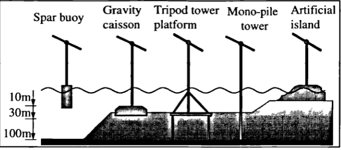
Spar buoy Gravity Tripod tower Mono-pile Artificial caisson platform tower island

lOmJ 3OmIf iOOml

Figure 1-1 Some offshore turbine concepts

The gravity caisson scheme has been widely publicised and was employed in the famous 'Vindeby' wind farm off the coast of Denmark. (Wind Engineering2 and Barthelmie3). Here the water depth is very shallow (2.1 - 5.1 m). In similar water depths the Dutch have sited a wind farm that uses a mono-pile foundation where the tower is effectively continued into the seabed and acts as a support pile. The concept adopted will depend greatly on the water depth in the chosen location. Figure 1-1 illustrates the water depths appropriate to each design. The floating concepts require water depths greater than 30m for an effective mooring system to be provided.

With the increasing size and complexity of the turbines comes a need for more flexible design tools to model the structural performance. hi the case of floating turbines is the additional necessity to determine the sea keeping ability and the effect of rigid body motions on the turbine loads. There are two methods of evaluating the response to the turbulent loads:

1. Time history analysis (time domain)

2. Power spectral density analysis (PSD frequency domain)

The time domain method involves the creation of a typical time history of the fluctuating sea and wave conditions. This is then passed through a dynamic simulation computer program that evaluates the time history of the platform motions and turbine stresses. Although this is a thorough method it has a number of disadvantages, in particular the time taken to perform a representative time analysis can be quite considerable and there is also difficulty in choosing an appropriate time history to apply to the structure. A number of scenarios should be applied to cater for the many loading combinations and conditions which affect the structure. These will include the

(29)

worst sea / wind combination and the general conditions that influence the fatigue life of the structure. Each scenario will require an additional calculation and each calculation will be computationally intensive and time consuming. For these reasons the frequency domain is often more appropriate, especially for preliminary scoping and optimisation calculations.

The PSD effectively represents the energy content in the wind and waves at a particular frequency. This is based on statistical measurements. The spectral models used for the wind and wave loading are based on the ESDU4 and Pierson Moskowitz5 spectra respectively. The power of the frequency domain lies in its calculation speed. Assuming that the structure behaves in a near-linear way enables the engineer to calculate a structural transfer function to model the structure. Applying additional loading scenarios is then a simple matter of multiplying each loading PSD by the transfer function. This simple and rapid calculation allows the engineer more potential to optimise the structure in the early stages of design. This is particularly appealing where fatigue is an important design issue because fatigue optimisation is not possible in the time domain due to the calculation time and expense involved. Time domain calculations are typically restricted, therefore, to verification exercises carried out at the end of the design phase.

1.2 Statement of the problem

If offshore floating turbine concepts are to be fully realised it is necessary to develop mathematical models that are able to rapidly predict the dynamic loads on the various components. Floating wind turbines are subjected to numerous random loading conditions from the wind and waves. To analyse the dynamic response from these it proves much faster to use an approach based in the frequency domain in the first instance.

(30)

dynamic behaviour and can lead to reduced design costs and better optimised schemes.

To properly analyse the response of a floating offshore turbine it is necessary to address three questions:

1. To what extent will the platform move in the water due to the combined wind and wave loading? (Equilibrium rigid body motion analysis.)

2. What effect do these platform motions have on the structural loading of the turbine?

3. What effect does the wind turbulence have directly on the structural loading of the turbine?

Having determined platform motions and the structural loads we can carry out seakeeping analyses and fatigue life prediction.

Only question 3 has been properly addressed and only recently have people even begun to consider the effect of structural dynamics and flexibility in the frequency domain. Garrad Hassan and Tecnomare UK Ltd. (Tong & Cannell') have considered Questions 1 and 2 but only for the simple case of surge motion.

This thesis derives a new analysis technique for addressing the three questions. This is an original piece of work and for the first time includes a 6-degree of freedom rigid body platform motion analysis and multi-degree of freedom structural finite element analysis.

1.3 The objectives of the study

The objectives of the study are to develop frequency domain analysis techniques for modelling wind turbine structures that are subjected to random wind loads and wave induced motions. In particular the analysis of floating offshore wind turbines.

(31)

determines the rotor loading on the structure. An analysis is then performed to evaluate mass, damping and stiffness matrices for the rigid rotor in 6 degrees of freedom. These describe the response of the rigid rotor as it is moved through the air along with the platform motion. The Super Element can be incorporated into existing analysis packages, such as AQWA6, to perform seakeeping analyses. This takes the sea elevation spectra and the wind turbulence loading spectra calculated by the Super Element and computes the 6 degree of freedom motion response of the vessel in terms of auto- and cross-power spectral densities.

The second stage takes the PSD of the turbulent wind speed along with the auto- and cross-power spectra of platform motion and computes the loads on the flexible turbine structure. This model includes all the structural flexibilities in the blades, tower and drivetrain.

The two stage approach is valid because structural flexibilities have been found to be insignificant in affecting the platform's motion, therefore a much simpler rigid body analysis ('Super Element') is suitable for this stage which can easily be incorporated into existing commercial software packages.

At the onset of this study, little development had been carried out on modelling the structural dynamics of a turbine in the frequency domain. Software packages from ECN7 (The Netherlands Energy Research Foundation) and Garrad Hassan Ltd. were available but these were limited in analysing only the turbulent wind loads on rigid turbine structures. It was therefore necessary to develop a new structural dynamic analysis in the frequency domain with the ability to analyse blade, tower and drivetrain flexibilities before progressing to include the rigid body motions.

1.4 Scope and limitations

The work derives mathematical models to predict the random loads on a turbine structure resulting from random wind speed and platform motion. All calculations are based in the frequency domain.

(32)

1. The derivation of a new structural analysis procedure to model the behaviour of flexible turbines in the frequency domain. These can be used for both on and offshore turbine analysis.

2. The derivation of a new rotor 'Super element' to model the response of a rigid turbine rotor to base motions and calculate the rotor loading due to turbulent winds. This 'Super Element' is used for seakeeping analyses. 3. The derivation of a new procedure to calculate the dynamic loads on a

flexible turbine blade subjected to rigid body motions and turbulent winds. This is used for structural analysis and design and for fatigue analysis using the latest frequency domain techniques.

1.5 Organisation of the Thesis

The thesis is organised as follows: chapters 2 to 4 detail the fundamental background on which the thesis is based. Chapter 2 discusses the theory of frequency domain analysis of multiple correlated random loads. It derives key relationships and formulae that are used throughout this text. Chapter 3 discusses the physical principles and theory behind the turbulent wind. It highlights the state of the art knowledge and the problems that face the offshore engineer. A thorough description of the ESDU 4 model is presented. Chapter 4 derives the state of the art aerodynamic analysis used in this project and comments on its limitations.

(33)

were performed in collaboration with WS Atkins Ltd. who are currently using the techniques for analysing existing and proposed turbine concepts.

Chapters 9 to 11 deal with the analysis of floating offshore turbines. Chapter 9 derives a rigid body model of the rotor to predict the reaction loads that arise when the rotor is moved through space in 6 degrees of freedom. This new 'Super Element' can be incorporated into existing hydrodynamic analysis packages, such as AQWA 6, to perform sea keeping analyses on the platform. Chapter 10 derives a new blade model that predicts the blade forces arising when the turbine is moved through space in 6 degrees of freedom. This is complicated because of additional harmonics that occur in the loading. A description is given on how this model is incorporated in the new finite element analysis technique derived earlier. Chapter 11 introduces a simple case study using a 'Tensioned Buoyant Platform (TBP)' on which is mounted a single wind turbine. TBP's serve as very stable platforms to mount offshore turbines and are renowned for their small dynamic motion response. The simplicity of the dynamic behaviour is highlighted and design conclusions made.

Chapter 12 presents the conclusions drawn from each chapter and suggests future work to be carried out.

1.6 Description of computer programs developed in this research

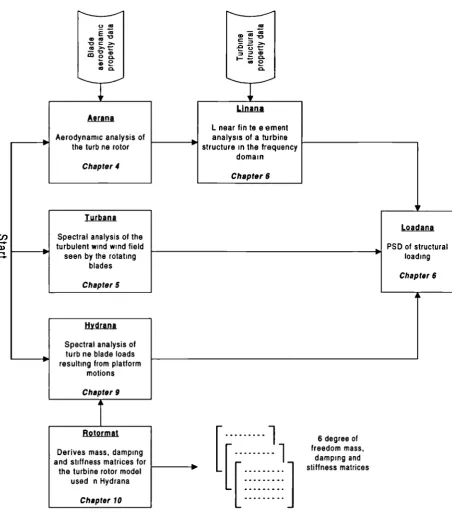
Computer programs have been developed as part of this research and these are referred to throughout the thesis. The computer programs are written using Mathcad versions Plus 5 and Plus & and is in a modular format with each module performing a particular analysis related to a chapter in the thesis. An overview of the modules is shown in Figure 1-2. Several modules are currently being used by WS Atkins Ltd.

(34)

o m ID = ID > ID 0. Aerana

Aerodynamic analysis of the turb ne rotor

Chapter 4 ID E>. 0. a. Llnana

L near fin te eement analysis of a turbine structure in the frequency

domain

Chapter 6

Turbana C1 Spectral analysis of the

__________ turbulent wind wind field seen by the rotating

blades

Chapter 5

Hydrang

Spectral analysis of turb ne blade loads resulting from platform

motions

Chapter 9

Rotormat

Derives mass, damping and stiffness matrices for

the turbine rotor model used n Hydrana

Chapter 10

Loadang

PSD of structural loading

Chapter 6

[...1

i r

1

freedom mass,

[

I dampin9 and

[ [

] stiffness matrices

Figure 1-2 Flow chart of Mathcad modules used in this research

'Tong K and Cannell C. (1993). "Technical and economical aspects of a floating offshore windfarm." Proceedings of a BWEAIDTI seminar, Cockroft Hall, Harwell, June 1993.

2

"Vindeby Offshore Windfarm." Wind Engineering, Volume 17 No. 3. 1993.

(35)

ESDU data sheets 82026 (1982), 85020 (1993) and 86010 (1991). "Strong winds in the atmospheric boundary layer. Parts I, II and III." ESDU International plc. London.

Pierson W.J and Moskowitz L. (1964). "A proposed spectral form of fully developed wind seas based on the similarity theory of S.A Kitaigorodskii." Journal of Geophysics. Res., Vol. 69.

6

Technical Manual to the AQWA-SUIT. Defraction analysis package. WS Atkins Ltd., Woodcote Grove, Ashley Road, Epsom, Surrey, England.

(36)

(37)

2. Frequency domain representation of random processes

2.1 Fourier series and the Fourier transform pair

2.1.1 Representing a time signal using Fourier series

Any periodic time history may be represented by the summation of a series of

sinusoidal waves of various amplitude, frequency and phase. This is the basis of

Fourier series expansion. A detailed explanation is given in Kreyszig' chapter 10. The

Fourier series expansion of a time history y(t) is often expressed by Equation 1.

"2,zn \

y(t) = A+Aco —._{tI+B sinl_.t)}}

í "

where

A0 = - fy(t)dt

A = . Jy(t) cos( —tjdt2,zn Ti

2 .12,zn

B =- Jy(t)sinl—.tjdt

'T I

T = period

Equation 1 Fourier Series Expansion

The terms A, A and B are termed Fourier coefficients and provide information on

the frequency content of the time history. A0 represents the mean of the time history

while A and B,, represent the amplitude of the various cosine and sine waves which

when added together comprise the time history. Figure 2-1 shows the Fourier series expansion for a particular saw tooth time history. By the third summation the

expansion is seen to give a reasonable representation of the original time history.

(38)

Ong nal time hstory

02

0I

Founer series 1st term

Penodl=I Mean Ao =0 041

02

A0+A 1 +B 1 +A2+B2+A3+B3

A -0 I B1 A0+A1+B1

Founer series 2nd term

°°2J\MWMAJ

°°5ltMV\AAMP

--

0 02

A2

-

005 B2 A0+A1 +B 1 +A2+B2

Founer series 3rd term

001

-001

A3

0.05

Ivvviis

-

005

B3

Figure 2-1 Fourier series expansion of a time history

The integrals within A and B effectively act as a filter and extract the amplitude of a

cosine or sine wave of frequency n/I' Hz. from the time history. This is accomplished

using the relationships given in Equation 2.

(2,zrnt" (2,znt

Jcosi )cos(%, )dt=

T T

TI

' . (2iimt' . (2,znt"i

Isini Isini idt=

'..

TI '.. tI

(2,zmt . (2nnt'\

Icosi Isini idt=

TI 'TI

O for m^n

1/2 for m=n

}

(39)

2.1.2 The complex Fourier series

In practice the Fourier coefficients A0, A and B prove very cumbersome to manipulate algebraically. Complex number theory helps with this aspect as all three coefficients may be replaced by one complex coefficient C. Many texts derive the complex Fourier series in detail, notably Kreyszig' chapter 10.6 and Barltrop2 chapter

3.3.3. However since a thorough understanding of it is so crucial to the research described a short derivation is given in this chapter.

The first thing to realise is that the sum of a cosine and sine wave results in a sinusoidal wave of amplitude r and initial phase angle 4 provided both waves have the same frequency. Figure 2-2 shows the summation of a cosine and sine wave with amplitudes A and B respectively and frequency (0.

01

- 005

0I

I

₀₀₄₇

+rv\iv\_—01 J\i

0069

\NVV

—0.1

A.cos(co.t) + B.sin(w.t) = r.cos(0.t +

Where r is the amplitude of the resultant sinusoidal wave and ₄is the initial phase offset

Figure 2-2 Summation of cosine and sine waves

The amplitude r and initial phase angle 4) of the resultant sinusoidal wave can be

obtained using the relationship given in Equation 3.

,=.,jA2+B2 Equation 3

(40)

40

?=IAI and where A = - tB,,

Equation 4

Having expressed the amplitude and initial phase of the sinusoidal wave in complex

terms it is now convenient to utilise the complex form of the exponential function to

represent the frequency term. This technique is explained in Kreyszig' chapter 2.3,

and follows the relationship given in Equation 5.

Equation 5

(2,, '\

±'l— " (2;izn \_ . (2in '

e " T

cosi • r + sin' t

T i I

Using these relationships the original Fourier term

(2 . ,r . n '\ 12•,rn "

Co t I + B . sin1 t I can be replaced with the complex number

T _{) "} T ₎

representation given in Equation 6.

Equation 6

ii. n _'I

(2•ir•n

)+B .(2 12''F 1

CO5

T

•

T

.tJ = T

Equation 1 may therefore be written in complex form by Equation 7.

I (2,r•n\

y(t) = A0 + A e T J

In-I

Equation 7

Where A =A—i•B

The expression may be simplified further by the introduction of negative frequencies.

These have the effect of cancelling the imaginary components in Equation 7 without

using the 9 { } function. Using the concept of negative frequencies Equation 7 can be

(41)

(2,r.n\ el—I: y(t)= Ce' T 1

n--Equation 9 Double sided Fourier series Equation 8 __

(2,rn\

4—): =

y(t)=A0+)Ae T +%Ae T

n-I n--I

where A = A - i B

Changing the limits of the summation the Fourier coefficients A0 and A can be replaced with the single complex Fourier coefficient C as expressed in Equation 9.

Where _{C =x(A.}

_iBn)=+1y(t).e{T)dt

Equation 9 is said to be double sided because it uses both positive and negative frequencies to represent the Fourier coefficients. Figure 2-3 shows a plot of the Real and Imaginary parts of the complex Fourier coefficients C, obtained from the expansion of the saw tooth wave in Figure 2-1. These are plotted with respect to frequency n/f Hz.

-fn

Re(C)

005

Real part of complex coefficient

lm(C)

004

1A

it\f\/1

oa

004

Imaginary part of complex coefficient

Figure 2-3 Plot of Real and Imaginary parts of complex Fourier coefficient

The complex Fourier coefficient C is used to obtain the amplitude and phase of the nth sinusoidal wave using the formulation given in Equation 10.

Amplitude r,, _V'nI+ICnIphase = ZC,, Equation 10

(42)

2.1.3 The Fourier density coefficient

Section 2.1.2 introduced the complex Fourier series expansion. For the analysis work covered in this thesis we are particularly interested in obtaining the complex Fourier coefficients. Each Fourier coefficient C, is obtained for a frequency of nIT Hz. The

frequency interval between each coefficient Af is therefore lIT Hz. This causes problems as the frequency at which the coefficients are calculated is dependent on the period T chosen. It is common practice to normalise the coefficients to eliminate the

dependence on T. The normalised coefficients take the form of a 'density function' and the Fourier coefficient is obtained from the area under the density curve for the range Af in question. This is shown in Figure 2-1.

Fourier density coefficient

Lf

-f f _{frequency Hz}

Figure 2-4 Fourier Density Coefficients

Using this normalisation the complex Fourier series expansion given in Equation 9 can be expressed by Equation 11.

(2 r y(t) = 4f. ±cII

T

A (2ffn\ where c = Jy(t) . etr)dt

Equation 11

and Af

The amplitude and phase of the sinusoidal wave with frequency _fis now obtained by taking the magnitude and argument of the area under the density curve in the region

Af. The function behaves much like a Probability Density Function.

(43)

the complex Fourier series is now expressed in integral form as Equation 12. This is

known as the Fourier Transform Pair. For future reference in this thesis 51(f) shall be

called the "Fourier Spectrum."

y(t) = Jy(f)

Inverse Fourier

-Transform

where 5(f) = Jy(t) . e 2 'cit

Founer Transform

Equation 12 Fourier Transform Pair

It is worth noting that many references use a different nonnalisation to that given

above. A common normalisation is to use the square root of the period. In this thesis

the form defined above shall be used.

2.1.4 The Fourier transform pair

The 'Fourier Transform Pair' was derived in section 2.1.3 in integral form and is

expressed in Equation 12. It is now apparent that a time history y(t) can be completely

expressed by the "Fourier Spectrum" y(f). The Fourier spectrum can therefore be

thought of as another 'frequency domain' in which a time history may be expressed.

In this sense 51(f) implies a description of the time history 'y' in the frequency

domain 'f . The 'Fourier Transform Pair' effectively transformations between the two

domains.

In addition to the integral form, the 'Fourier Transform Pair' can also be described in

a discrete form. This is particularly beneficial as most measured time histories are

obtained in a discrete, digitised form with values taken over equally spaced intervals

in time. In these circumstances the integral form is difficult to process and it is

desirable to perform some numerical routine on the measured time history to

(44)

Fourier transform." The result obtained from a discrete transformation will tend to the result obtained from an integral transformation as the sample length and sampling frequency increase.

Cooley and Tuke? devised a very rapid discrete Fourier transform algorithm in 1965. It is known as the "Fast Fourier Transform (FFT)" and has a reverse process called the "Inverse Fourier Transform (Jk'F!)." There are a number of derivatives of these each using a different normalisation, it is important therefore to check software literature before implementing commercial computer routines. The norrnalisaiion proposed in this thesis is chosen to give the same result as that obtained with the integral form. The "Discrete Fourier Transform Pair" is defined in Equation 13.

(2,rk'

y(tk) = !. e''

T

3(ffl)=—•y(tk).e N

Inverse Fourier Transform Fourier Transform

Equation 13 Discrete Fourier transform pair

The Fast Fourier Transform is only applicable for data containing exactly 2' data points, where m is any integer number greater than 1. For this reason it is standard practice to subdivide the digitally recorded time history into buffers containing 2m data points then evaluate the Fourier transform on each separately. As a result of the buffering then a number of issues such as windowing, overlapping and zero padding also become an issue, these are also discussed by Newland4, chapters 10 to 11, and the author in his lecture on the frequency domain, Halfpenn. We are not concerned with the discrete algorithm in this thesis and the reader is referred to the above references for more details.

2.1.5 Fourier analysis of random time histories

(45)

statistics are not affected by a shift in the time origin. (i.e. the statistics of a time history X(t) are the same as a time history X(t + t) for all values of t) To test for stationarity we take a number of recordings of the random process at different times. The process is stationary if the probability distributions of the ensemble are the same for all points in time. If the ensemble probability density function is Gaussian then the process is known as a Gaussian random process. A stationary process is called an ergodic process if statistics taken from one sample are the same as those obtained for the ensemble. With an ergodic stationary random process, therefore, we can effectively take a single sampled time history from the process and safely assume that this contains all the required statistical properties of the parent process. For nonstationary processes the statistics obtained from a sampled time history would not be representative of those of the whole random process as these would be continuously changing. Priestley6, chapter 3, and Newland4 discuss stationarity at length and the reader is referred to these texts for more information. The analysis of nonstationary random processes is not considered in this thesis. However it does become a problem for the offshore wind farm designer because offshore wind is typically nonstationary. This is discussed later in Chapter 3.2. Further information on analysing nonstationary processes is given in Priestley6 chapter 11.

(46)

Random time history

time

5

frequency Hz

Imaginary part of Fourier spectrum

110

5 FFT —>

<— IFFT

Real part of Fourier spectrum

frequency Hz

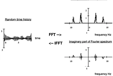
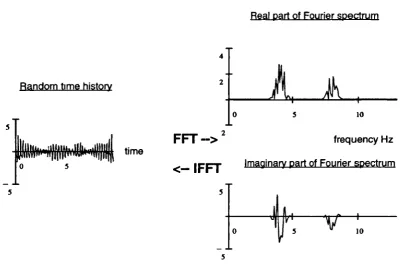
Figure 2-5 Frequency domain representation of a random time history

For real time histories the Fourier transform is symmetric about zero Hz. A Double

Sided Spectrum is said to be symmetric if the relationships given by Equation 14 are satisfied.

9{5(f)} = Equation 14

= I{— 5;(_f)}

It is usual to express a symmetric spectrum as a "Single Sided Spectrum." The "Single Sided Spectrum" contains the same information as the "Double Sided Spectrum" but is often more convenient to use because negative frequencies are not considered. All measured time histories can be expressed as a Single Sided Spectrum. The relationship between single and double sided spectra is given by Equation 15.

7(f) =2•5D(f) Equation 15

(47)

Random time history

4

2

Real part of Fourier spectrum

FFT-->2 frequency Hz

time

<— IFFT Imaginary part of Fourier spectrum

frequency Hz

Figure 2-6 Single sided Fourier transform

2.1.6 Power spectral density function (PSD)

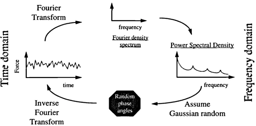
Previously in this thesis we have considered the representation of a time history in the frequency domain. Often it is more beneficial to have a statistical description of the time history than the deterministic one and for this purpose the "Power Spectral Density (PSD)" function is useful. A description is said to be deterministic when one can determine the actual value given by the process at any point in time. A time history is deterministic because the value can be obtained by observing the plot at the required instance in time. Likewise the Fourier spectrum is also deterministic because all the amplitude, frequency and phase information is retained and can be transformed back into the corresponding time history. The disadvantage of the Fourier spectrum is in the complex manner with which the amplitude and phases are stored. For an ergodic stationary Gaussian random process, it has been observed that the phases angles are purely random with a constant probability distribution between —7t and +it.

(48)

Spence7 provides a very good historical and qualitative description of history of the PSD and how to interpret its results.

The PSD gives a statistical representation of a stationary random process in the frequency domain. It is defined such that the area beneath the PSD represents the mean square amplitude of the random process. This normalisation proves very beneficial as is demonstrated later. Many design standards, such as the ESDU 8 papers on wind turbulence, express the statistical properties of random processes in terms of PSDs. Using these in conjunction with a linear structural model allows PSDs of structural stresses and deflections to be calculated and fatigue life estimates to be obtained. These subjects are covered later in the thesis. The PSD is used in the same way as the Fourier Density spectra. The mean square amplitude of a sinusoidal wave of frequency! can be obtained by taking the sum of the area under the PSD at +f and _-f over the interval i&f as Ef—+O. This is illustrated in Figure 2-7. The mean amplitude of

the component sinusoidal waves over frequency Ef is obtained by taking the square root of twice the mean squared values.

-f f _{frequency Hz}

Figure 2-7 Double sided power spectral density (PSD)

PSDs may be complex and expressed as both double or single sided spectra in the same way as the Fourier density spectra. The relationships given in Equation 14 and Equation 15 hold for single and double sided PSDs. PSDs calculated from measured time histories will always be real. Complex PSDs however are encountered later in the thesis. The real part of a complex PSD SW is known as the co-spectral density function P(f) and the imaginary part as the quad-spectral density Q(f).

(49)

frequency range Af is obtained from the Fourier spectra by taking the modulus of the area under the curve as expressed in Equation 16.

Amplitude(f) = Af 5(f) Equation 16

The area under a PSD represents the mean squared amplitude of the component sinusoidal waves where Mean Square(f) = -• Amplitude

2

. We can equate the mean square amplitudes calculated from the PSD and the Fourier spectra and hence determine the transformation between the two; this is derived in Equation 17.

4f.G(f)=+.Ef2 Equation 17

The double sided PSD is determined in a similar fashion, the results are summarised in Equation 18.

S(f)

=.I

D (f)I

2

or _{S(f) = (YDf 5D(f)) for double sided PSDs or}

G(f) = _{(f)I or G(f) = -(}

y

_{(f) . y5 (f))}

for single sided PSDs

Where yD(f) is the complex conjugate of YD(J).

Equation 18

Both the modulus and complex conjugate forms of the transformations are correct however it is mathematically beneficial to use the complex conjugate form. It is also worth noting that many books adopt a different notation for the double and single sided PSDs. In this thesis the notation SW and G(f) is adopted for the double and single sided spectra respectively. In later chapters we also use radian measure and express frequency in terms of ai radians per second.

Section 2.1.3 commented on the use of different normalisations applied to the Fourier transform. It is quite common to see the JT normalisation being used and this changes

(50)

the formulation expressed in Equation 18 to the form

S(f)

_{= ID(f)I}

_{2 or}

S(f) =

(f)

YD

(f)).

The normalisation chosen for the Fourier transform is not

important provided that the resultant PSDs are the same.

The PSD provides considerable information about the statistics of the random process. By definition the area under the PSD represents the mean square amplitude of the time history, the root mean squared (RMS) of the time history is therefore determined as the square root of this. This is the single most important quantity in random process theory. Other statistical properties may be obtained using the spectral moments of the PSD. The nth spectral moment m of a PSD is defined by Equation 19.

Equation 19 m{S(f)} =

JS(f) . f"df

The key statistical properties listed in Equation 20 were derived by S.O. Rice9 in

1954. These properties become important when considering the fatigue life of a structure. This is explained in detail in Chapter 7.

Root Mean Square (RMS)

₀

=

Expected number of upward zero

E[o]

crossings m0

Expected number of positive peaks

E] =

Irregularity factor - E[O]

E[p]

Equation 20 Statistical properties of a PSD (after SO. Rice9)

(51)

as broad or wide band, which is introduced later. For narrow band histories j' - 1 whereas for broader band yreduces and tends to zero.

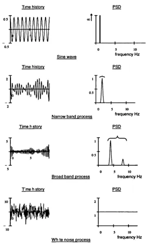
The appearance of the PSD plot also conveys much information. Figure 2-8 shows four types of process. The distinction between narrow and broad banded processes becomes much more apparent from the PSD plots than the time histories. This is illustrated in Figure 2-8.

Time history PSD

TI1M'V

ccl

I I

0.5

0 5 10

Sine wave frequency Hz

Time history PSD

0 5 10

Narrow band process frequency Hz

Time hstory PSD

05

)

A,

Broad band process frequency Hz

Wh te noise process

Tmehstorv PSO

2

I I

0 5 10

frequency Hz

(52)

A sine wave of frequency! is shown in the frequency domain as a single spike centred atf The area under the spike yields the mean squared amplitude of the sine wave and the amplitude may therefore be detennined by taking the square root of twice this value. In theory the spike will be infinitely narrow as the sine wave has a single finite frequency. As the PSD is a density function, the spike will therefore have an infinite height. This situation is described by Dirac's delta function, which is described later in the thesis. In practice we usually employ a numerical solution technique for determining the PSD, such as the FFT; this will give a finite frequency resolution and so the spike will never be infinite.

The narrow band time history comprises a number of component sinusoidal waves over a narrow range of frequencies. The PSD shows this situations quite clearly. This type of time history is usually typified in the time domain by a low frequency envelope known as the 'beat effect'.

A wide band time history comprises a number of component sinusoidal waves over a wide range of frequencies. Again the PSD shows this situation quite clearly. This type of time history is usually typified in the time domain by having many valleys occurring above the mean and many peaks occurring below the mean. In contrast, the narrow band time histories demonstrate most of the peaks falling above the mean and subsequent valleys falling approximately the same distance below the mean. The irregularity factor, 2' is therefore a useful parameter for determining how 'wide banded' a signal is. For narrow band signals y -* 1, while for wide band signals y -0.

A white noise signal is formed by the summation of an infinite number of sinusoidal waves of the same amplitude and random phase. The PSD of this signal clearly shows uniform amplitude content at each frequency.

2.1.7 Time signal regeneration from PSDs

In section 2.1.2 it was shown that a stochastic or random process may be expressed in

(53)

process in the frequency domain and in many instances it is desirable to obtain a time history from a PSD.

Unlike the Fourier density spectra the PSD does not contain information about the phase relationships between the sinusoidal waves that make up the time history. It does however contain information on the Mean square amplitude of each wave. In order to regenerate a time history it is necessary to reintroduce the phase relationships between each of the waves. For many signals it has been found that the phase relationships follow a uniform random distribution between - and r radians and with this knowledge it is therefore possible to regenerate a time history. Time histories obeying this trend are said to be Gaussian Random processes. The regenerated time history will not be the same as the original measured time history because the phase angles are now different, however it is still statistically equivalent. There are a number of methods used for time history regeneration from PSDs. The author describes a method he employed for "nCode International' 0" that uses the PSD to calculate a digital filter by which to filter a white noise signal and hence obtain the desired frequency response. This chapter looks at the more intuitive method of evaluating the random phase angles and taking the inverse Fourier transformation.

The time history is formed by the summation of a number of sinusoidal waves of differing frequency, amplitude and phase. The nth wave may be expressed in the form given in Equation 21.

= • cos(v . t + where is the random phase angle

between 0 and n radians.

Equation 21

Dynamic analysis of both on and offshore wind turbines in the frequency domain

Wind Turbines in the Freq uency Domain

by

Andrew Halfpenny

A Dissertation submitted for the degree of Doctor of Philosophy in

Faculty of Engineering, University of London

University College London

Department of Mechanical Engineering

February 1998.

Acknowledgements

Abstract

Contents

List of Figures

List of tables

Nomenclature

c)

s

t

=

i{x}

c(o)

(f)

Jt

(t)

t,

1. Introduction

[...1

i r

1

2. Frequency domain representation of random processes

°°2J\MWMAJ

°°5ltMV\AAMP

--

-

Ivvviis

-

TI '.. tI

I

\NVV

1A

it\f\/1

2

=.I

2

y

(f) . y5 (f))

S(f)

2 or

S(f) =

(f)

(f)).

JS(f) . f"df

0

TI1M'V

A,

_t

_(f)

_{(f) . y5 (f))}

_{2 or}

₀