Uncertainty Quantification for a Class of MEMS-based Vibratory Angular Rate Sensors

(1)

Western University Western University

Scholarship@Western

Electronic Thesis and Dissertation Repository

8-14-2014 12:00 AM

Uncertainty Quantification for a Class of MEMS-based Vibratory

Angular Rate Sensors

Nujhat Abedin

The University of Western Ontario

Supervisor

Dr. S. F. Asokanthan

The University of Western Ontario

Graduate Program in Mechanical and Materials Engineering

A thesis submitted in partial fulfillment of the requirements for the degree in Master of Engineering Science

Follow this and additional works at: https://ir.lib.uwo.ca/etd

Part of the Acoustics, Dynamics, and Controls Commons, and the Electro-Mechanical Systems Commons

Recommended Citation Recommended Citation

Abedin, Nujhat, "Uncertainty Quantification for a Class of MEMS-based Vibratory Angular Rate Sensors" (2014). Electronic Thesis and Dissertation Repository. 2245.

https://ir.lib.uwo.ca/etd/2245

This Dissertation/Thesis is brought to you for free and open access by Scholarship@Western. It has been accepted for inclusion in Electronic Thesis and Dissertation Repository by an authorized administrator of

(2)

i

Uncertainty Quantification for a Class of

MEMS-based Vibratory Angular Rate Sensors

By

Nujhat Abedin

Graduate Program in Engineering Science

Department of Mechanical and Material Engineering

Submitted in partial fulfilment

of the requirements for the degree of

Master of Engineering Science

School of Graduate and Postdoctoral Studies

The University of Western of Ontario

London, Ontario, Canada

August 2014

(3)

ii

ABSTRACT

Numerical schemes that are suitable for predicting response statistics of mass-spring and ring

gyroscopes are developed when this class of vibratory gyroscopes are subjected to certain system

parameters as well as environment uncertainties. The emphasis is placed on the steady-state part

of the response since it is more critical to the operation of a gyroscope. A peak-picking approach

which simulates the demodulation process which is used in practice is employed first before

applying the Monte Carlo simulation method to predict the response statistics. A number of

simulation trials to predict response statistics have been performed for mass-spring and ring-type

gyroscopes in an effort to ascertain the optimal temporal points as well as sample paths for the

impending uncertainty quantification study. Based on the optimal temporal and sample paths,

uncertainties in input angular rate, mass/frequency mismatch and damping have been quantified.

Keywords: MEMS based gyroscope, General coordinate, Uncertainty quantification, Monte

Carlo method, Numerical prediction, Ensemble mean, Mass mismatch, Frequency mismatch,

(4)

iii

ACKNOWLEDGEMENTS

This thesis would not have been come to light without the cooperation of the my thesis

supervisor Dr. S. F. Asokanthan. I am deeply thankful to him for introducing me to this research

area and for his continuous guidance, encouragement and expertise and valuable contribution to

this thesis.

I would like to express my gratitude to those who provided me with guidance and support during

the course of this thesis. My thanks also go to my colleagues and friends for their helpful and

friendly behavior.

I would like to express special thanks to Dr. Quazi Mehbubar Rahman and Muhammad Bashar

for their guidance and inspiration.

Finally, I would like to thank organizations such as the National Sciences and Engineering

Research Council (NSERC) of Canada discovery grant, The University of Western Ontario's

Academic Development fund/Small Grants and Western Graduate Research Scholarship

(WGRS) from the University of Western Ontario, as this research work was partly funded by

(5)

iv

The work is dedicated to my beloved mother Zinnat Zahanara

I am who I am because of my mom

(6)

v

List of Tables

Table 2- 1. Parameters of Mass-spring Gyroscope for the Numerical Simulations ... 18

(10)

ix

List of Figures

Figure 1-1. Analog MEMS Vibratory Gyroscope (reproduced from Giunta at el., 2006) ... 3

Figure 1-2. Delphi‘s metal ring gyroscope (reproduced from the website of Silicon Sensing

Systems Japan Ltd.) ... 4

Figure 2-1. Translation-based single-axis vibratory gyroscope ... 13

Figure 2-2. Motion of a particle in body-fixed frame that rotates relative to an inertial frame .... 14

Figure 2-3. Radial displacement in the (a) driving direction and (b) sensing direction without

input angular rate ... 20

Figure 2-4. Input angular rate time-profile ... 22

Figure 2-5. Radial displacement in the (a) driving direction and (b) sensing direction with

𝛺 = 2π rad/sec input angular rate ... 23 Figure 2-6. Variation of radial displacement in the (a) driving direction and (b) sensing direction

when frequency mismatch values change from 0 to 0.03% while one frequency is fixed another

is changing for 𝛺 = 2π rad/sec input angular rate ... 25 Figure 2-7. Time response after peak-picking for mass-spring gyroscope (𝛺=2𝜋 rad/sec) ... 30 Figure 2-8. Number of points (time) Vs Mean along the time response for mass-spring gyroscope

(a) without drift (b) with drift (𝛺=2𝜋 rad/sec) ... 32 Figure 2-9. Number of points Vs standard deviation along the time response for mass-spring

gyroscope (a) without drift (b) with drift (𝛺=2𝜋 rad/sec) ... 33 Figure 2-10. Radial displacement in the sensing direction with input angular rate (100 samples)

... 34

Figure 2-11. Number of samples Vs Ensemble Mean (a) without drift and (b) with drift (100

samples along path axis and 𝛺=2𝜋 rad/sec) ... 35 Figure 2-12. Number of points Vs Standard deviation (a) without drift and (b) with drift (100

samples along path axis and 𝛺=2𝜋 rad/sec) ... 36

(11)

x

Figure 3-3.Number of samples along path axis Vs Ensemble mean (a) without drift and (b) with

drift (𝛺=2𝜋 rad/sec) ... 41 Figure 3-4. Number of samples along path axis Vs Standard deviation (a) without drift and (b)

with drift (𝛺=2𝜋 rad/sec) ... 42 Figure 3-5. Radial displacement in the sensing direction with input angular rate at point 4501 (50

samples) ... 43

Figure 3-6. Standard deviation of input angular rate vs. standard deviation of output response,

(frequency mismatch is 0.01%) ... 47 Figure 3-7. Standard deviation of frequency mismatch vs. standard deviation of output response,

(𝛺 = 2𝜋 rad/sec) ... 48 Figure 3-8. Standard deviation of frequency mismatch vs. standard deviation of output response,

(𝛺 = 2𝜋 rad/secand 𝑄 = 1000) ... 49 Figure 3-9. Standard deviation of quality factor mismatch vs. standard deviation of output

response for different frequency mismatch (𝛺 = 2𝜋 rad/sec) ... 50 Figure 3-10. Standard deviation of quality factor (non-dimensional) vs. standard deviation of

output response for fixed frequency mismatch (𝜗 = 0.01%, 𝛺 = 2𝜋 rad/sec) ... 51 Figure 3-11. Variation of amplitude ratio for different input angular rates (frequency mismatch

with 0.01%, Quality factor, 𝑄𝑥 = 𝑄𝑦 = 1 × 108)... 54 Figure 3-12. Variation of amplitude ratio for different input angular rates (frequency mismatch

with 0.01% mismatch, Quality factor, 𝑄𝑥 = 𝑄𝑦 = 1000) ... 54 Figure 3-13. Variation of frequency response for different input angular rates (frequency

mismatch with 0.01% mean, Quality factor, 𝑄𝑥 = 𝑄𝑦 = 1 × 108) ... 55 Figure 3-14. Variation of frequency response for different input angular rates (frequency

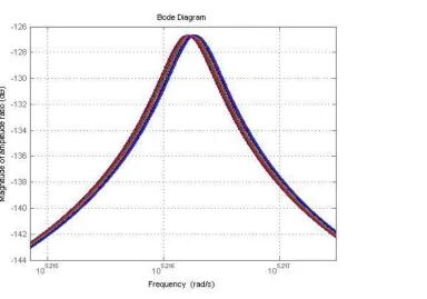
mismatch with 0.01% mean, Quality factor, 𝑄𝑥 = 𝑄𝑦 = 1000) ... 55 Figure 3-15. Variation of amplitude ratio for different samples (frequency mismatch with 0.01%,

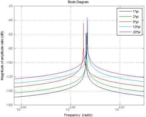
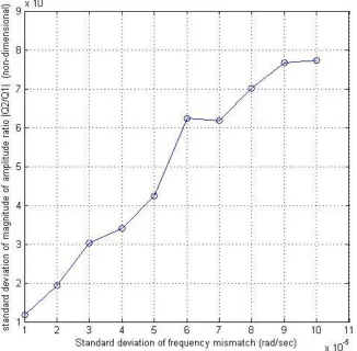
Quality factor, 𝑄𝑥 = 𝑄𝑦 = 1000, 𝛺 = 2𝜋 rad/sec) ... 56 Figure 3-16. Standard deviation of frequency mismatch vs. standard deviation of magnitude of

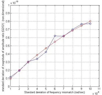
amplitude ratio 𝑄2/𝑄1 (𝛺 = 2𝜋 rad/sec, Quality factor, 𝑄𝑥 = 𝑄𝑦 = 1000) ... 57 Figure 3-17. Standard deviation of frequency mismatch vs. standard deviation of magnitude of

(12)

xi

Figure 3-18. Standard deviation of frequency mismatch vs. standard deviation of frequency of

peak amplitude ratio 𝑄2/𝑄1 (𝛺 = 2𝜋 rad/sec, Quality factor, 𝑄𝑥 = 𝑄𝑦 = 1000) ... 59

Figure 3-19. Standard deviation of input frequency mismatch vs. standard deviation of magnitude of frequency response 𝑄2/𝐹1 (𝛺 = 2𝜋 rad/sec, Quality factor, 𝑄𝑥 = 𝑄𝑦 = 1000) ... 60

Figure 3-20. Standard deviation of frequency mismatch vs. standard deviation of magnitude of frequency response 𝑄2/𝐹1 (𝛺 = 2𝜋 rad/sec, Quality factor, 𝑄𝑥 = 𝑄𝑦 = 1000) ... 61

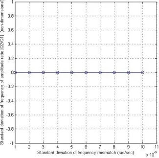
Figure 3-21. Standard deviation of frequency mismatch (rad/sec) vs. standard deviation of frequency of frequency response 𝑄2/𝐹1 (non-dimensional) (𝛺 = 2𝜋 rad/sec, Quality factor, 𝑄𝑥 = 𝑄𝑦 = 1000) ... 62

Figure 4-1. Schematic of a rotating ring with support springs ... 65

Figure 4-2. Stationary flexural modes of a rotating ring with n=2, 3, 4 nodal diameters ... 66

Figure 4-3. Second flexural modes used in the normal mode equations ... 67

Figure 4-4. Radial displacement in the (a) driving direction and (b) sensing direction without input angular rate ... 74

Figure 4-5. Input angular rate time-profile ... 76

Figure 4-6. Radial displacement in the (a) driving direction and (b) sensing direction with input angular rate for 𝛺 = 2𝜋 input angular rate ... 77

Figure 4-7. Variation of radial displacement in the driving (a) and sensing (b) directions for different mass mismatch values ... 79

Figure 4-8. Time response after peaks-picking for ring gyroscope (𝛺=2𝜋 rad/sec) ... 81

Figure 4-9. Number of points vs Mean along the time response for ring gyroscope (a) without drift (b) with drift (𝛺=2𝜋 rad/sec) ... 83

Figure 4-10. Number of points vs standard deviation along the time response for ring gyroscope (a) without drift (b) with drift (𝛺=2𝜋 rad/sec) ... 84

Figure 4-11. Radial displacement in the sensing direction with input angular rate (100 samples) ... 85

(13)

xii

Figure 4-13. Number of points vs Standard deviation (a) without drift and (b) with drift (100

samples along path axis and 𝛺=2𝜋 rad/sec) ... 87

Figure 5-1. Time response after peak-picking for ring gyroscope (Ω=2π rad/sec) ... 91

Figure 5-2. Radial displacement in the sensing direction after peak-picking (70 samples) ... 91

Figure 5-3. Number of samples along path axis vs. Ensemble mean (a) without drift and (b) with

drift (𝛺=2𝜋 rad/sec) ... 93 Figure 5- 4. Number of samples along path axis vs. Standard deviation (a) without drift and (b)

with drift (𝛺=2𝜋 rad/sec) ... 94 Figure 5-5. Radial displacement in the sensing direction with input angular rate at point 6201 (70

samples) ... 95

Figure 5-6. Standard deviation of input angular rate vs. standard deviation of output response,

(mass mismatch is 0.01%) ... 97 Figure 5-7. Standard deviation of mass mismatch vs. standard deviation of output response,

(𝛺 = 2𝜋 𝑟𝑎𝑑/𝑠𝑒𝑐) ... 98 Figure 5-8. Standard deviation of mass mismatch vs. standard deviation of output response,

(𝛺 = 2𝜋 𝑟𝑎𝑑/𝑠𝑒𝑐) ... 99 Figure 5-9. Standard deviation of damping ratio mismatch vs. standard deviation of output

response for different mass mismatch (𝛺 = 2𝜋 𝑟𝑎𝑑/𝑠𝑒𝑐, 𝜉 = 0.01) ... 101 Figure 5-10. Standard deviation of damping ratio vs. standard deviation of output response for

different mass mismatch (𝛺 = 2𝜋 𝑟𝑎𝑑/𝑠𝑒𝑐, 𝜉 = 0.01) ... 102 Figure 5-11. Variation of amplitude ratio for different input angular rates (mass mismatch with

0.01%, damping ratio, 𝜉=1× 10 − 9) ... 104 Figure 5-12. Variation of amplitude ratio for different input angular rates (mass mismatch with

0.01% mismatch, damping ratio, 𝜉=0.01) ... 105 Figure 5-13. Variation of frequency response for different input angular rates (mass mismatch

with 0.01% mean, damping ratio, 𝜉=1× 10 − 9) ... 105 Figure 5-14. Variation of frequency response for different input angular rates (mass mismatch

(14)

xiii

Figure 5-15. Variation of amplitude ratio for different samples (frequency mismatch with 0.01%,

damping ratio, 𝜉=0.01, 𝛺 = 2𝜋 𝑟𝑎𝑑/𝑠𝑒𝑐) ... 107 Figure 5-16. Standard deviation of mass mismatch vs. standard deviation of magnitude of

amplitude ratio 𝑄2/𝑄1 (𝛺 = 2𝜋 𝑟𝑎𝑑/𝑠𝑒𝑐, damping ratio,𝜉=0.01) ... 108 Figure 5-17. Standard deviation of mass mismatch (non-dimensional) vs. standard deviation of

magnitude of amplitude ratio 𝑄2/𝑄1 (𝛺 = 2𝜋 𝑟𝑎𝑑/𝑠𝑒𝑐, damping ratio, 𝜉=0.01) ... 109 Figure 5-18. Standard deviation of mass mismatch vs. standard deviation of frequency of

amplitude ratio 𝑄2/𝑄1 (𝛺 = 2𝜋 𝑟𝑎𝑑/𝑠𝑒𝑐, damping ratio, 𝜉=0.01) ... 110 Figure 5-19. Standard deviation of input mass mismatch vs. standard deviation of magnitude of

frequency response 𝑄2/𝐹1 (𝛺 = 2𝜋 𝑟𝑎𝑑/𝑠𝑒𝑐, damping ratio, 𝜉=0.01) ... 111 Figure 5-20. Standard deviation of input mass mismatch vs. standard deviation of magnitude of

frequency response 𝑄2/𝐹1 (𝛺 = 2𝜋 𝑟𝑎𝑑/𝑠𝑒𝑐, damping ratio,𝜉=0.01) ... 112 Figure 5-21. Standard deviation of mass mismatch vs. standard deviation of frequency of

(15)

xiv

Nomenclature

𝛺 Input angular rate (rad/sec)

𝑣 Radial velocity (m/s)

𝐹𝑟 Force in radial direction (N)

𝐹𝜃 Force in tangential direction (N)

r Radial displacement mass-spring gyroscope (m)

𝑚_𝑝 Proof mass (non-dimensional)

𝐶_𝑥 Viscous damping constant along x-axis (Ns/m)

𝐶_𝑦 Viscous damping constant along y-axis (Ns/m)

𝑘_𝑥 Linear spring constant along x-axis (N/m)

𝑘_𝑦 Linear spring constant along y-axis (N/m)

𝐹 Harmonic driving force (N)

𝜔𝑥 x-axis natural frequency (rad/sec)

𝜔_𝑦 y-axis natural frequency (rad/sec)

Q Quality factor (non-dimensional)

𝑄𝑥 x-axis quality factor (non-dimensional)

𝑄𝑦 y-axis quality factor (non-dimensional)

𝑀 Mass matrix

𝐺 Gyroscopic matrix

𝐷 Damping matrix

(16)

xv

𝒒 Generalized coordinate vector

𝑞1 Generalized coordinate vector along x-axis (m) for mass-spring

gyroscope

𝑞₂ Generalized coordinate vector along y-axis (m) for mass-spring gyroscope

𝑞1, 𝑞2 Generalized coordinates corresponding to the flexural mode for ring

gyroscope

𝑞₃, 𝑞₄ Generalized coordinates corresponding to the circumferential mode for

ring gyroscope

𝛺 Steady-state angular speed (rad/sec)

𝜍₁ Drift coefficient

𝜍2 Uncertainty coefficient

𝑎𝑑 Drift exponential coefficient

𝜉 Damping ratio (non-dimensional)

𝜗 Frequency mismatch parameter (non-dimensional)

𝜍𝑟𝑒𝑠𝑝𝑜𝑛𝑠𝑒 Standard deviation of output response (m)

𝜍𝑓.𝑚𝑖𝑠𝑚𝑎𝑡𝑐 𝑕 Standard deviation of frequency mismatch (rad/s)

𝜍𝑞.𝑚𝑖𝑠𝑚𝑎𝑡𝑐 𝑕 Standard deviation of quality factor mismatch (non-dimensional)

𝐹₁ 𝑠 Laplace transform of 𝑓₁ 𝑡

𝑄1(𝑠) Laplace transform of 𝑞1(𝑡)

𝑄2(𝑠) Laplace transform of 𝑞2 𝑡

(17)

xvi

𝜃

Angle of separation between a set of degenerate modes (rad)

𝛾 and 𝜅₂ Constant (non-dimensional)

𝜅1 Angular rate (rad/sec)

ζ(𝑡) Random component (dependent on uncertain variable)

𝜔01 Non-rotating ring natural frequency associated with the flexural

generalized coordinates 𝑞₁ (rad/sec)

𝜔02 Non-rotating ring natural frequency associated with the flexural

generalized coordinates 𝑞2 (rad/sec)

𝜌 Density (Nickel) (𝑘𝑔/𝑚3)

𝐸 Young's Modulus (Nickel) (𝑁/𝑚2)

r Mean Radius of ring (𝜇𝑚)

𝑕 Radial Thickness of ring (𝜇𝑚)

𝑏 Axial Thickness of ring (𝜇𝑚)

𝛿𝑚 Mass mismatch (non-dimensional)

𝜍𝑚.𝑚𝑖𝑠𝑚𝑎𝑡𝑐 𝑕 Standard deviation of mass mismatch (non-dimensional)

(18)

1

Chapter 1 1. Introduction and literature review

1.1. Introduction

MEMS (Micro-Electro-Mechanical Systems) based inertial sensors, namely the accelerometer

and the gyroscope, have gained much attention in the past few years. These devices have

found several useful engineering applications that include spacecraft orientation, vehicle stability

control, navigation assist, vehicle roll over detection, image stabilization and cellular phones.

Current MEMS gyroscopes are lighter and compact. They utilize less power and therefore, are

considered to provide a cost-effective solution when compared to the moderately priced

spinning-disk mechanical gyroscopes and the expensive Fiber-optic as well as Ring Laser

gyroscopes.

The design methodologies for MEMS devices are based on deterministic approaches, where the

input parameters, for example geometrical and physical properties are assumed to be known

precisely. However, in practice, due to the batch-production processes used in MEMS

fabrication as well as the micron-scale dimensions of the structural elements, consideration of

uncertainties in system parameters and an understanding of their effects are warranted. Hence,

the primary purpose of the present thesis is to develop a systematic process for uncertainty

quantification based on the dynamic response.

All MEMS based gyroscopes that have been developed thus far are based on internal vibratory

(19)

2

two types vibratory MEMS gyroscopes are considered in the present thesis, namely the

mass-spring type vibratory gyroscope and the ring-type gyroscope. In order to predict response

statistics, for both MEMS gyroscopes, in time as well as in the frequency domain, numerical

schemes are developed from suitable mathematical models. In the interest of examining the

effect of randomness on output responses, random inputs are introduced in the numerical

schemes in the form of noise and drift terms. Monte Carlo method is employed in the

simulations for predicting the response statistics. Based on these numerical schemes uncertainty

quantification is performed via quantifying standard deviations of output responses, when both

mass-spring and ring gyroscopes are subjected to parameter uncertainties. It is envisaged that

this quantitative understanding will lead to improved performance of this class of gyroscopes.

1.2. Literature review

MEMS gyroscopes include the micromechanical and electronic parts which have been fabricated

on a single chip (see, e.g., Geen at el., 2002 and Lai at el., 2009). For this class of gyroscopes,

the batch production with low cost and high precision is a target in the future. The

implementation used thus far for the MEMS gyroscopes utilize a vibratory configuration where

the Coriolis effect is exploited for the precise sensing of angular rotation rates. Different types

of micromachined structures can be used as the vibratory elements in the design of angular rate

sensors, including prismatic beams, tuning forks, single or dual masses, disks, and rings (see e.g.,

(20)

3

Mechanical coupling between the drive and detection modes of a single mass-spring

micro-machined-vibrating gyroscope was studied by Mochida, Tamura and Ohwada (2000) giving

importance to the mechanical coupling. A suitable mathematical model for a dual axis

gyroscope was proposed by Davis (2001). Davis represented an accurate model for the single

mass-spring gyroscope by considering the coupling effect for both the driving and sensing axes.

Figure 1-1 shows a typical configuration for mass-spring gyroscope where the effective spring

supports have been represented by the thin beams, and the mass situated in the middle is referred

to as the proof mass which is capable of vibrating in the plane of the structure. This proof mass

is subjected to oscillation in a plane along one axis (driving axis), and if the device is subjected

to a rotational motion about an axis orthogonal to this plane, as a result of the Coriolis effect, the

proof mass will tend to oscillate in the same plane along an axis referred to as the sensing axis

which is orthogonal to the driving axis. The input angular rate can be determined by measuring

the motion along the sensing axis.

Figure 1- 1. Analog MEMS Vibratory Gyroscope (reproduced from Giunta at el., 2006)

Bifurcation behaviour of a single-axis mass-spring MEMS gyroscope has been studied by Wang

(2009) considering nonlinear stiffness elements when the input angular rate of this system is

(21)

4

paths for both sub-harmonic and combination resonance cases have been formulated and

examined by employing the method of averaging as well as a numerical approach.

In the case of ring-type gyroscopes, models to study in-plane vibrations of a rotating ring has

been developed and represented by Bickford and Reddy (1985). The effects due to shear

deformation and rotary inertia for higher rotational speeds and for higher bending modes were

demonstrated. Huang and Soedel (1987) also investigated the in-plane vibrations of rotating

rings. In particular, variations of natural frequencies and mode shapes influenced by rotational

speed and elastic supports were examined. The research presented by Putty and Najafi (1994)

provided information of a vibrating ring gyroscope in which the ring structure is driven into

resonance in the plane of the chip and provided suitable design details. Delphi reported about a

vibratory ring gyroscope using electroplated metal to form a ring structure on top of

complementary metal-oxide semiconductor (CMOS) chips (see, Sparks et al. 1999). A scanning

electro-micrograph (SEM) of the device is shown in Figure 1-2. Semicircular springs support

the ring and stored the vibration energy. The spring design has greater effect of packaging

stresses on the sensor.

(22)

5

Ring gyroscope has balanced symmetrical structure which is less sensitive to environmental

vibrations. Since two identical flexural modes of the structure are used to sense rotation, the

sensitivity of the sensor is amplified by the quality factor of the structure. Ring gyroscope is less

temperature sensitive while two flexural vibration modes are equally affected by temperature

(see, e.g., Putty, 1995). However, the ring structure is known to be more resistive to ambient

vibrations (see, e.g., Lee, et al, 2011).

A suitable mathematical model for examining the stability and response of a rotating ring

perturbed by periodic fluctuations were developed by Cho (2004). For the purpose of

investigating the dynamic behaviour of a ring gyroscope, the reduction of the equations of

motion to a suitable discrete linear form is performed first. Under external excitation and body

rotation, time and frequency responses for varying parameter values of damping and input

angular rate with the effects due to ring asymmetry were quantified. The ring gyroscope model

used in the present thesis is based on the above research.

The practical application of the Monte Carlo Simulation (MCS) method is based on the fact the

next best situation to having the probability distribution of a certain random quantity is to have a

corresponding large population. The execution process of the method consists of numerically

simulating a population corresponding to the random quantities in the physical problem, solving

the deterministic problem associated with each member of that population, and obtaining a

population corresponding to the random response quantities. This population can then be used to

get statistics of the response variables (see e.g., Ghanem and Spanos, 2012).

The Monte Carlo method is a quite versatile mathematical tool having the ability of handling

(23)

6

various fields such as health care, agriculture, and econometrics. However, in engineering

mechanics it has attracted intense attention only recently following the universal availability of

low-cost computational systems. The computational availability has caused an interest in

developing sophisticated and efficient simulation algorithms. Shinozuka and Jan (1972) have had

a pioneering role in introducing the method to the field of engineering mechanics. Most of the

applications of the MCS have been in the study of random variation of deterministic media (see

e.g., Ghanem and Spanos, 2012). Generating samples to create the response surface is a very

important part of the uncertainty quantification process and there are a number of ways to do it.

Though one can again use the Monte Carlo approach, significant gains are to be had by sampling

more intelligently (see e.g., Snow and Bajaj, 2010). In their study, MCS has also been

successfully employed in understanding the uncertainty quantification in a MEMS switch. An

efficient stochastic framework for quantifying the effect of stochastic variations in various

design parameters on the performance of MEMS devices has been performed by Agarwal and

Aluru (2009). The above two studies limit their analysis to static behavior as well as spatial

co-ordinates.

Following the above research on the use of Monte Carlo Simulation to MEMS devices for

uncertainty quantification, the research performed in the present thesis, unlike the previous

studies focuses on the prediction of response statistics of MEMS gyroscopes based on the

(24)

7

1.3. Motivation

The application of MEMS vibratory gyroscopes are expanding from consumer electronics to

aerospace and are now one of the most common MEMS products. In many applications,

consumers demand MEMS gyroscopes that are reliable even in rough environments. Some of

these harsh environments include high temperature, high humidity, high-G mechanical

shock/drop, high mechanical vibration, high frequency acoustic noise, high radiation, high

magnetic and electric field. In many applications like navigation and tracking, deep water

energy exploration, down-hole drilling and high-temperature industrial applications, the MEMS

gyroscope sensor experiences temperatures that are beyond the manufacturer‘s recommended

temperature range. In this type of environment, the device is likely to be subjected to

environmental uncertainties that may adversely affect the performance, reliability as well as

durability. To investigate the performance characteristics of MEMS gyroscopes by using

laboratory experiments to simulate the above environmental conditions usually expensive and

time-consuming. Thus, a simulation approach is preferred.

A sensor such as a rate gyroscope can directly measure the angular velocity of a rotating body

without a need for processes such as integration (of angular acceleration) or differentiation (of

angular displacement). In general, the performance level of gyroscopes can be classified into

three different categories: rate-grade, tactical-grade and inertial-grade. The inertial grade can be

considered as the most accurate and sensitive while the other two classes are listed in the order of

lower accuracy and sensitivity. Until now, although many types of micro-machined vibratory

gyroscope have been proposed and developed as inertial sensors, to date the performance level of

(25)

8

appropriate for long-term operations or for a signal integration process since they possess

significantly high drift error as well as noise. Thus, it is clear that many challenges are ahead for

the design of MEMS gyros in order that their performance levels can be increased to those

offered by conventional rate-grade gyros, and to achieve tactical and inertial-grade performance

level (see e.g., Cho, 2004). Drift and noise are random in nature and to predict the effects of drift

on MEMS gyroscope one of the appropriate ways is to employ the Monte Carlo method to

numerically simulate the response of MEMS gyroscopes using suitable mathematical models.

The manufacturing tolerances in MEMS are notoriously poor and additionally the effects that

parameters variations have on device behaviour are poorly understand. The result is that

gyroscope performance and life time are difficult to control or predict. Understanding the effects

of these deviations is important for predicting the ranges of performance exhibited by a

manufactured product can vary significantly from that of the nominal design. Uncertainty

Quantification also permits prediction of device yield and is a first step towards predicting

gyroscope lifetime.

In order to address some of the limitations proposed above, an uncertainty quantification study is

proposed. Extensive studies on the dynamics and uncertainty quantification of different system

as well as environmental parameters associated with MEMS inertial sensors, it is envisaged that

(26)

9

1.4. Aims of the thesis

The primary intent of the present thesis is to predict dynamic response behaviour of mass-spring

as well as ring gyroscopes when subjected to an angular motion and perform an uncertainty

quantification study for quantifying the effect of parameter uncertainties. To this end, Monte

Carlo simulation is used to compute the response statistics as well as for determining a suitable

measure. To date, a systematic procedure for performing this analysis is not available, hence the

results and the procedures to be developed is envisaged to pave the way towards future research

in this area. To achieve this objective, the following steps are considered:

 Develop a numerical scheme based on a suitable mathematical model for systematic

characterization of mass-spring gyroscopes giving emphasis to uncertainty quantification.

 Develop a numerical scheme based on a suitable mathematical model for systematic

characterization of ring gyroscopes giving emphasis to uncertainty quantification.

 Develop a systematic process to illustrate the optimal temporal as well as sample paths

for predicting output statistics in time domain as well as frequency domain via Monte

Carlo method for both types of gyroscopes.

 Perform uncertainty quantification analysis for mass-spring gyroscope based on output

response statistics in time domain as well as in the frequency domain when the system is

subjected to uncertainties in angular rate, quality factor and frequency mismatch. A

suitable measure for characterizing this uncertainty is also expected.

 Perform uncertainty quantification analysis for ring gyroscope based on output response

(27)

10

of input angular rate, damping ratio and mass mismatch. A suitable measure for

characterizing this uncertainty is also proposed.

1.5. Thesis Outline

This thesis mainly focuses on two types of gyroscopes namely, the mass-spring gyroscope and

the ring-type gyroscope. It may be noted that the methodology applied for both types of

gyroscopes are the same and for this reason readers will find similarities in paragraphs, sentences

and phrases in Chapters 2 and 4, and also in Chapters 3 and 5.

In Chapter 2, a mathematical model for the mass-spring gyroscope for the purposes of dynamic response predictions are introduced and discussed. When the gyroscope is subjected input

angular rotation, dynamic response analysis is performed to characterize the dynamic behavior of

mass-spring system in time domain via suitable numerical schemes. Time response analyses are

preformed, and are examined for cases without and with drift. Monte Carlo simulation method is

applied to achieve optimal characteristics for the output response statistics which are suitable for

further analyses.

Chapter 3 discusses briefly the results obtained via the numerical simulations performed in the previous chapter for the mass-spring gyroscope. The effect of varying input angular rate,

frequency/stiffness mismatch and quality factor for the mass-spring gyroscope due to presence of

noise and drift in the system are obtained and discussed. This analysis forms the basis for the

uncertainty quantification study based on the response statistics and are expressed in terms of the

(28)

11

examined next and the results are discussed in terms of the peak magnitude statistics associated

with amplitude ratio as well as the forced response.

In Chapter 4, a mathematical model for the ring-type gyroscope for the purposes of dynamic response predictions are introduced and discussed. When the gyroscope is subjected input

angular rotation, dynamic response analysis is performed to characterize the dynamic behavior of

mass-spring system in time domain via suitable numerical schemes. Time response analyses are

preformed, and are examined for cases without and with drift. Monte Carlo simulation method is

applied to achieve optimal characteristics for the output response statistics which are suitable for

further analyses.

Chapter 5 discusses briefly the results obtained via the numerical simulations performed in the previous chapter for the mass-spring gyroscope. The effect of varying input angular rate, mass

mismatch and quality factor for the ring gyroscope due to presence of noise and drift in the

system are obtained and discussed. This analysis forms the basis for the uncertainty

quantification study based on the response statistics and are expressed in terms of the input and

the output standard deviation. Uncertainty quantification in the frequency domain is examined

next and the results are discussed in terms of the peak magnitude statistics associated with

amplitude ratio as well as the forced response.

Chapter 6 presents the conclusions based on the response and uncertainty quantification results for the mass-spring and ring-based vibratory angular rate sensors, along with contributions, and

(29)

12

Chapter 2 2. Dynamic Response Analysis for Mass-Spring Gyroscopes

2.1. Introduction

In this chapter, numerical schemes that are suitable for simulating the time-domain dynamic

behavior of mass-spring type vibratory gyroscopes are developed. These schemes are intended

for the purpose of uncertainty quantification and, in particular, for the purpose of predicting the

dynamic behavior of this class of devices under uncertain environment as well as system

parameters. To this end, a mathematical model is used to represent the dynamic behavior of a

translation-based single-axis mass-spring gyroscope and in particular a model presented by

Davis (2001) is adopted. For the purposes of characterizing the behavior due to uncertain system

as well as environmental parameters of mass-spring type gyroscopes, steady state portion of

transient responses are employed. In order to examine the effects of randomness on the MEMS

gyroscope response, Monte Carlo simulation method is used for estimating the ensemble mean

as well as the standard deviation (measure of variance) of response samples. The propagation of

mean and standard deviation are investigated so that optimal as well as robust sampling

strategies can be developed based on the simulated dynamic responses. These strategies as well

as suitable sample selections form the basis of further uncertainty quantification to be performed

(30)

13

2.2. Model description

Mass-spring gyroscope model used in the present thesis is based on the equations developed by

Davis (2001) and later presented in the work by Tianfu Wang (2004) and Ye Tian (2005). The

gyroscope configuration consists of a lumped point mass (proof mass) at the center and four

springs that support the mass as shown in Figure 2-1. It may be noted that the proof mass type

general configuration can represent several practical vibrating gyroscope designs that have been

used in MEMS fabrications. In order to achieve maximum sensitivity, this gyroscope is excited

at a resonant drive frequency, along the x-axis in steady-state (driving direction), while the input

angular rate 𝛺 is introduced along the z-axis (input axis) which is orthogonal to the driving axis.

Owing to the Coriolis effect that result from velocity along the x-axis and frame rotation rate 𝛺 along the z-axis, the lumped proof mass oscillates along the direction of y-axis which is referred

to as the sensing axis. It may be noted that the mass is confined to oscillate in the x-y plane at all

times and the steady oscillatory motion along the sensing axis is used as a basis for the

measurement of the angular rate ' 𝛺 '.

(31)

14

2.3. Equations of Motion

It is known that Coriolis acceleration plays a significant role in governing the dynamics of this

class of gyroscopes that are of interest to the present thesis. A rigid body is considered to be

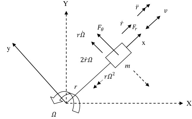
subjected to Coriolis acceleration when it moves with a velocity with respect to a rotating frame

of reference. If a body of mass m is considered to move along the x-axis with a velocity 𝑣, this acceleration component is represented as 2𝛺 × 𝑣, where the body fixed-frame x-y-z rotates at an angular velocity 𝛺 about a fixed frame of reference (inertial frame) X-Y-Z as shown in Figure 2-2.

Figure 2-2. Motion of a particle in body-fixed frame that rotates relative to an inertial frame

Equations that govern the motion of this body when subjected to forces 𝐹_𝑟 and 𝐹_𝜃 in the

directions shown in Figure 2-2 can be derived as: 𝑚 𝑟 − 𝑟𝛺2 = 𝐹_𝑟,𝑚 𝑟𝛺 + 2𝑟 𝛺 = 𝐹_𝜃. The

𝑟𝛺2_{term represents the centripetal acceleration, while the}_{2𝑟 𝛺}_{term represents the Coriolis}

acceleration in accordance with the vector product 2𝛺 × 𝑣 described earlier. The terms 𝑟 and 𝛺 , respectively, are the radial and tangential acceleration.

𝑣

Y

𝐹𝑟

𝐹𝜃

x y

m r

X

𝛺

𝑟 𝑟

2𝑟 𝛺

𝑟𝛺

(32)

15

Based on a linear model that represents a harmonically excited gyroscopic system by Wang and

Asokanthan (2009), the homogenous system of equations that represent the free motion is

formulated as follows

𝑚𝑥 + 𝐶𝑥𝑥 + 𝑘𝑥𝑥 − 𝑚𝛺2𝑥 − 2𝑚𝛺𝑦 − 𝑚𝛺 𝑦 = 0, (2.1)

𝑚𝑦 + 𝐶_𝑦𝑦 + 𝑘_𝑦𝑦 − 𝑚𝛺2_{𝑦 + 2𝑚𝛺𝑥 + 𝑚𝛺 𝑥 = 0,}_(2.2)

where 𝑥, 𝑦 represent the system generalized coordinates, while 𝑚 represents the proof mass.

𝑘_𝑥 and 𝑘_𝑦 denote the linear spring constants while 𝐶_𝑥 and 𝐶_𝑦 are the viscous damping constants.

Here, the gyroscope is considered to be subjected to an input angular rate 𝛺 about the Z-direction. It may be noted that the motion along the z-axis is decoupled from the motion along x

and y axes and hence are not considered to be important for the present analysis.

When the gyroscope is subjected to a harmonic force 𝐹 = 𝐹₀𝑠𝑖𝑛 𝜔_𝑥𝑡 along the driving direction (i.e., x-axis), the equations of motion for this gyroscopic configuration can be obtained as

𝑥 +𝜔𝑥

𝑄𝑥𝑥 − 2𝛺𝑦 + 𝜔𝑥

2_{− 𝛺}2_{𝑥 − 𝛺 𝑦 =} 𝐹0

𝑚𝑝𝑠𝑖𝑛 𝜔𝑥𝑡, (2.3)

𝑦 + 2𝛺𝑥 +𝜔𝑦

𝑄𝑦 𝑦 + 𝛺 𝑥 + 𝜔𝑦

2 _{− 𝛺}2_{𝑦 = 0,}_(2.4)

where 𝐹₀represents the excitation force magnitude, 𝑚_𝑝 the mass of the gyroscope proof-mass

while 𝜔_𝑥 and 𝜔_𝑦 represent, respectively, the undamped natural frequencies associated with the x

(33)

16

by 𝑄𝑥and 𝑄𝑦 while 𝛺 represents the angular rate of the rotating frame of reference, which is

essentially the angular rate signal to be sensed by the gyroscope.

The governing equations (2.3) and (2.4) can then be written in matrix form as follows:

𝑀𝒒 + (𝐺 + 𝐷)𝒒 + 𝐾𝒒 = 𝐹 (2.5)

where, 𝒒 = [𝑥 𝑦]𝑇 = [𝑞₁ 𝑞₂]𝑇 represents generalized coordinate vector, and the system matrices are defined as

𝑀 = 1 0_{0 1} , 𝐺 = 0_2𝛺 −2𝛺₀ , 𝐾 = 𝜔𝑥2− 𝛺₀ 2 _𝜔 0

𝑦2− 𝛺2 , (2.6)

𝐷 =

𝜔𝑥

𝑄𝑥

0

𝜔𝑦

𝑄𝑦

, 𝐹 =

𝐹0

𝑚𝑝

𝑠𝑖𝑛 𝜔

𝑥

𝑡

0 ,

(2.7)

with

𝜔

_𝑥2

=

𝑘𝑥

𝑚

, 𝜔

𝑦2

=

𝑘𝑦

𝑚

, 𝑄

𝑥

=

𝑚𝜔𝑥

𝑐𝑥

, 𝑄

𝑦

=

𝑚𝜔𝑦

𝑐𝑦

.

Equations (2.5) are employed for the purposes simulating the time response analysis for fixed

system parameter values which is described in the following section. In addition these equations

are also suitably modified to accommodate uncertainties via random variation of parameters to

aid uncertainty quantification. The uncertainty results are presented partly in this chapter and in

(34)

17

2.4. Simulation of Deterministic Time Response

2.4.1. Introduction

In the present chapter, in order to investigate the dynamic characteristics of mass-spring

gyroscope time response analysis is performed considering the mathematical model derived in

the previous section. The time response analysis is then performed assuming that the mass is

excited with a periodic external force in which the excitation frequency is set to be the same as

the natural frequency associated with a non-rotating system so that the system gain can be

maximized. It may be noted that the natural frequency variation with the input angular rate has

been marginal and hence this choice for the excitation frequency is considered to have minimal

influence on resonance. The dynamic effects due to variation of typical parameters of a MEMS

mass-spring gyroscope are examined via numerical simulations and are depicted via suitable

transient response plots. Results for the varying system parameters such as the input angular

rate, damping and frequency/stiffness mismatch are then presented.

2.4.2. Numerical Simulations

In a mass-spring gyroscope, it is assumed that the mass-spring element is excited by a harmonic

external force while the gyroscope as a whole is subjected to an angular rate that is measured.

When the system is under the influence of typical input signals it is useful to perform a dynamic

response analysis for the mass-spring system. For this purpose, a numerical simulation

(35)

18

performed later in Chapter 3. The simulation is performed via the fourth-order Runge-Kutta

scheme available within the MATLAB computing environment.

Typical parameters associated with a MEMS-based mass-spring type gyroscope are considered

as shown in Table 2-1, for the purpose of numerical simulations.

Table 2-1. Parameters of Mass-spring Gyroscope for the Numerical Simulations

Proof mass 𝑚_𝑝 = 3.6 × 10−10 (𝑘𝑔)

x-axis natural frequency 𝜔_𝑥 = 164536 𝑟𝑎𝑑/𝑠𝑒𝑐 ≈ 26.2 (𝑘𝐻𝑧)

y-axis natural frequency 𝜔_𝑦 = 164536 𝑟𝑎𝑑/𝑠𝑒𝑐 ≈ 26.2 (𝑘𝐻𝑧)

x-axis quality factor 𝑄_𝑥 = 1000 (non-dimensional)

y-axis quality factor 𝑄_𝑦 = 1000 (non-dimensional)

The equations of motion (2.3) and (2.4) are written in the first order form that is suitable for

numerical integration of the ODE‘s as follows:

𝑞 ₁ = 𝑞₃, (2.8a)

𝑞 ₂ = 𝑞₄, (2.8b)

𝑞 ₃ = − 𝜔_𝑥2_{− 𝛺}2_𝑞

1+ 𝛺 𝑞2−𝜔_𝑄𝑥

𝑥𝑞3+ 2𝛺𝑞4+

𝐹0

𝑚𝑝𝑠𝑖𝑛 𝜔𝑥𝑡, (2.8c)

𝑞 ₄ = −𝛺 𝑞₁− 𝜔_𝑦2_{− 𝛺}2_𝑞

2− 2𝛺𝑞3−𝜔_𝑄𝑦

(36)

19

Equations (2.8) are implemented in MATLAB and fourth order Runge-Kutta scheme is

employed for integrating the set of ODE‘s. System parameter listed in Table 2-1 has been used

in the simulations while the two natural frequencies 𝜔_𝑥 and 𝜔_𝑦 along the x-axis and y-axis respectively are considered to be identical first to examine the behavior in the absence of

frequency/stiffness mismatch. The ODE45 integration routine has been found to be suitable for

the numerical simulations, with initial conditions set to be zero and the value of time step is set

to be 0.00001 seconds.

2.4.2.1. Time response without input angular motion

When the mass-spring system is subjected to harmonic excitation without any input angular

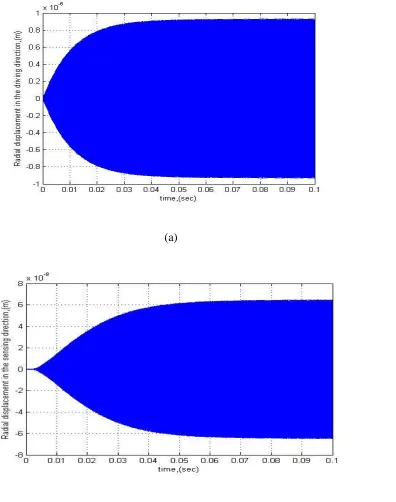
motion (𝛺=0 rad/sec), the response of the mass-spring gyroscope along the driving direction is achieved numerically and the results are illustrated in Figure 2-3 (a). It can be seen that the

vibration amplitude of the proof mass reaches a steady-state after about 0.04 seconds from the

commencement of the excitation. On the other hand, the response of the mass-spring gyroscope

(37)

20

(a)

(b)

(38)

21 2.4.2.2. Time response with input angular motion

It has been shown that the variations of natural frequencies with the input angular rates are

significantly small in the low speed range (i.e., less than 2π rad/sec) for which typical mass-spring gyroscopes are designed (Cho, 2004). Hence, the excitation frequency 𝜔 can be assumed to be constant and to coincide with one of the two non-rotating natural frequencies (say 𝜔𝑥

associated with the generalized coordinate x).

In order to examine the response of the mass-spring gyroscope associated with the generalized

coordinate 𝑞₂(sensing direction), a suitable profile for the input angular rate must be applied. In the present analysis, this profile is assumed to start from a zero value and reach a steady-state

angular speed 𝛺 via a smooth increase in speed as depicted in Figure 2-4. The equation used to represent an input angular rate profile that represents a smooth increase in the angular rate has

been chosen to be

𝛺 =

𝑛𝜋 2

sin(

𝜋𝑡 0.005

−

𝜋 2

) +

𝑛𝜋

2 for 𝑡 < 0.005 (2.9)

At time 𝑡 = 0.005 seconds the input angular rate time-profile is set to reach the steady-state. Different steady-state angular speeds can be used to investigate the dynamic response for

(39)

22

Figure 2- 4. Input angular rate time-profile

In this chapter, a steady-state angular speed of 𝛺 = 2𝜋 has been chosen for the purpose of illustrating typical dynamic responses. When both the input angular motion and the harmonic

excitation are introduced simultaneously, the time responses of the system in the driving and the

(40)

23

(a)

(b)

Figure 2-5. Radial displacement in the (a) driving direction and (b) sensing direction with

(41)

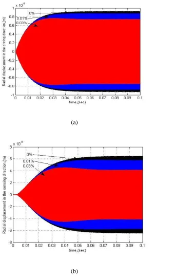
24 2.4.2.3. Frequency mismatch

Owing to the uncertainties present in the MEMS fabrication process, it is impossible to obtain

equal stiffness for the suspension elements in the x-y direction. This will manifest in the system

as a frequency mismatch for the driving and sensing motion. Hence, this form of

frequency/mass mismatch is considered as one of the important parameters that affect the system

dynamics significantly. Hence, the effects of frequency mismatch on the time response of the

mass-spring gyroscope are examined in this section. Figures 2-6 (a) and (b) show the response

amplitudes for the mass-spring system in the driving and sensing directions until t=0.1 seconds. It may be noted that although the simulation was performed for 0.2 seconds, for the purpose of

clear demonstration of the transient part of the response, only the response until 0.1 seconds has

depicted in the figures. As illustrated in Figure 2-6 (b), a reduction in the response in the sensing

direction is evident when the frequency mismatch of the vibratory system is increased. It may be

noted that this reduction can be detrimental to the achievable performance of this forms of

gyroscopes, e.g., it can lead to lower sensitivity for the angular rate sensor. Comparison of the

corresponding steady state responses in the driving and sensing directions indicate that this

mismatch causes relatively larger reductions in the response in the sensing direction. Further,

uncertainty propagation of the parameter can be considered to be important and forms a basis for

(42)

25

(a)

(b)

(43)

26

2.5. Simulation of Random Time Response

2.5.1. Introduction

In the present study, to see the effect of randomness and drift due to input angular rate and

certain important parameters of MEMS mass-spring gyroscope model, a drift noise model is

assumed in the form of an equation as

𝑑_𝑑 = 𝜍₁ 𝑒𝑎𝑑𝑡− 1 + 𝜍

2𝜁(𝑡) (2.10)

This model consists of two parts. The first part represents the drift, which is an exponential term,

while the second part denotes the uncertainty, which is a random component. In order to obtain

the typical drift rate from equation (2.10), the drift exponential coefficient 𝑎_𝑑 is set at a value 1.0 and the drift coefficient 𝜍₁ is set at a value 0.0245. Uncertainty coefficient 𝜍₂ is chosen to be 0.001.

For the present study, the model presented via Equation (2.10) is to represent additive noise and

drift to the nominal input angular rate 𝛺. Hence, the input angular rate takes the form:

𝛀 =𝛺 + 𝑑_𝑑 (2.11)

The drift/noise model presented in equation (2.10) is also employed for representing

uncertainties in other system parameters such as mass/frequency mismatch, and quality

(44)

27

2.5.2. Monte Carlo Simulation

As MEMS gyroscopes are developed using micro manufacturing technologies, micro scale

products usually have a relatively large manufacturing uncertainties compared to normal macro

scale products. Reduction of the variance of material properties as well as the geometric

properties of a micro scale product is quite expensive. The geometric and materials

uncertainties caused by a micro manufacturing process inevitably lead to the uncertainty of the

product performance. Therefore, to achieve a reliable design of a product, the performance

uncertainty of the product, which is often expressed by the variance or standard deviation, needs

to be estimated in a reliable way. Estimated standard deviation may prove to be useful in

quantifying the quality of the manufacturing product prior to determining the quality via testing

of product samples. Here, Monte Carlo simulation is used to aid prediction of the effects of

uncertainties so that metrics for the response standard deviation can be quantified.

Monte Carlo methods may vary from system to system but it has obviously followed a particular

pattern, such as, determination of a input domain, generation of random inputs with a probability

distribution, calculation of the results for many samples of the inputs and prediction of a suitable

measure of response statistics. Monte Carlo simulation relies on the process of precisely

representing uncertainties by specifying inputs as probability distributions. If some of the inputs

to a system are uncertain, the future performance must also be uncertain. That is, the result of

any analysis based on inputs represented by probability distributions is itself a probability

distribution.

Every Monte Carlo simulation starts off with developing a deterministic model which closely

(45)

28

nominal values (or the base case) of the input parameters are used. Mathematical relationships

are applied using the nominal values of the input variables, and transformed into the desired

output. After adequate performance from the deterministic models is predicted, the risk

components are added to the model. As mentioned before, since the risks originate from the

stochastic nature of the input variables, these variables are generated from suitable distributions.

A set of random numbers (also called random variates or random samples) are generated from

these distributions after identifying the underlying distributions. One set of random numbers,

consisting of one value for each of the input variables, will be used in the deterministic

model, to provide one set of output values. Then this process needs to be repeated to generate

more sets of random numbers, one for each input distribution, different sets of possible output

values must be collected. This part is the core of Monte Carlo simulation (see e.g.,

Raychaudhuri, 2008).

In this case input angular rate 𝛀 has been considered as a sample which contains the random

component ζ 𝑡 is presented in Figure 2-7. Monte Carlo method has been applied for many samples of input angular rate 𝛀. Owing to the presence of randomness, the simulations are run

repeatedly for randomly generated values for 𝛀. As a result, many several samples of output

responses are obtained for further analysis and the examination of useful measures of response

statistics forms the basis of the uncertainty quantification.

When the mass-spring system is subjected to uncertainties in input angular rate (𝛺), frequency (𝜔_𝑦) and quality factor (𝑄_𝑦), randomness is usually incorporated in those parameters and Monte

Carlo simulation is used to generate many output samples that correspond to uncertain input

(46)

29

2.5.3. Robustness of simulation

2.5.3.1. Stochastic response simulation after peak-picking

As demonstrated in section 2.4.2.2, the output time response in the sensing direction contains

two parts, namely transient and steady-state. The transient part of the time response changes

with time until it reaches the steady state. Since the steady-state part of the response is more

critical to the operation of a gyroscope, this part has been chosen for applying the Monte Carlo

method. Further, the high frequency oscillatory motion has been removed via a suitable

peak-picking method. Peak-peak-picking method is employed to find peak values of an oscillating

response. There are several processes to do peak-picking and in the present thesis, MATLAB

command 'findpeaks' is used to get peak values of the responses. The purpose of going through

this step is to simulate the demodulation process that is used in practice as part of

MEMS-gyroscope signal processing elements. This approach aids in quantifying the variation of the

mean values and the standard deviation of the steady state of time response along the sensing

direction. After peak-picking and the removal of the transient part, the resulting response is used

to characterize and predict response statistics via Monte Carlo method. The plot that represents

this response is illustrated in Figure 2-7 where the last sample point which is approximately

13,000 coincides with 0.5 seconds. In the next sections, an attempt will be made to justify the

(47)

30

Figure 2-7. Time response after peak-picking for mass-spring gyroscope (𝛺=2𝜋 rad/sec)

2.5.3.2. Optimal number of points along time response

Before performing the uncertainty quantification, it is important to come up with a suitable set of

data that exhibits consistence and convergence for the response statistics. For this purpose,

number of samples along the time axis as well number samples along the sample paths have been

considered. In this chapter, various time data sets as well as ensemble data sets have been

considered to establish a robust scheme for predicting useful response statistics. This has been

achieved primarily via examining the temporal mean, temporal standard deviation, ensemble

(48)

31

The ensemble average of a repetitive response is defined by defining a time for each path,

creating the ensemble of time varying signals referenced to that time and then averaging across

this ensemble at this time instant.

An attempt is made to define the number of points along the time axis which can be used for the

application of Monte Carlo method based on the numerical simulation. After peak-picking and

the removal of the transient, the first 100 points along the remaining steady state response shown

in Figure 2-7 has been considered first. These 100 points have been used to determine the

temporal mean and standard deviation. This process is considered with increments of 100 points

up to 6000 points. This process is performed for cases without and with the drift, keeping the

noise component the same.

Figures 2-8 and 2-9, respectively, illustrate the results for the temporal mean and the standard

deviation. These figures also illustrate that, reasonable convergence will be achieved after 2000

points which are considered for further analysis in predicting mass-spring gyroscope response

statistics. Figures 2-8 and 2-9 also illustrate the effect of increasing drift on the response

statistics. Hence, an alternate approach is warranted for predicting the response statistics for

(49)

32

(a)

(b)

(50)

33

(a)

(b)

(51)

34

The statistical response predictions performed in the previous section confirms the significance

of considering time sample points past the 2000 points based on both the mean and standard

deviation. In order to ascertain the predictions via the sample paths, 100 random samples have

been employed. The sample paths are depicted in Figure 2-10.

Employing the 100 samples, the ensemble mean as well as the standard deviations are computed.

Figures 2-11 (a) and (b), show the ensemble mean without and with drift. Figures 2-11 (a) and

(b) show that reasonable consistency for ensemble mean without drift is obtained for any points

after 3600 points and ensemble mean with drift shows no consistency. This may be attributed to

the effect of increasing drift on the response. However, the predictions made for the standard

deviations for the response are illustrated in Figures 2-12 (a) and (b). These figures demonstrate

that after 3900 points in cases without and with drift standard deviation values show a

converging trend and points past the 3900 mark may be considered suitable for further analysis

in predicting response statistics.

(52)

35

(a)

(b)

(53)

36

(a)

(b)

(54)

37 2.5.3.3. Discrete time steps

It is known that time step size plays a significant role in the numerical simulation process.

Obviously, smaller time steps results in more accurate predictions of the response along with

increased computations costs. In order to find the optimal time step to achieve reasonably

accurate results in moderate time, a suitable fixed step size is selected by running several

simulations via the ODE45 integration routine within MATLAB. Based on the simulation trials

the time step size has been chosen to be 0.000001 seconds. Further reduction in step size has

been found to be unnecessary.

2.6. Closure

A suitable numerical model is developed for investigating the dynamic response characteristics

of a mass-spring element when the mass-spring gyroscope is subjected to an input angular rate.

The natural frequency variations caused by gyroscopic coupling in the system matrix are

investigated. Time and frequency responses of the mass-spring gyroscope are examined when it

is excited by a harmonic external force while the sensor is subjected to an angular rate.

Response amplitudes are obtained when parameters frequency mismatch are varied. It is found

that the presence of noise and drift terms have effects on the mass-spring system. However,

randomness is introduced in numerical model to get the stochastic response. Different methods

are performed to achieve a robust scheme for predicting useful response statistics via Monte

Carlo simulation. These optimized response statistics are used in uncertainty quantification of

Uncertainty Quantification for a Class of MEMS-based Vibratory Angular Rate Sensors

Scholarship@Western

Scholarship@Western

Uncertainty Quantification for a Class of MEMS-based Vibratory

Uncertainty Quantification for a Class of MEMS-based Vibratory

Angular Rate Sensors

Angular Rate Sensors

Uncertainty Quantification for a Class of

MEMS-based Vibratory Angular Rate Sensors

ABSTRACT

ACKNOWLEDGEMENTS

Table of Contents

List of Tables

List of Figures

Nomenclature

𝜃

Chapter 1

1. Introduction and literature review

1.1. Introduction

1.2. Literature review

1.3. Motivation

1.4. Aims of the thesis

1.5. Thesis Outline

Chapter 2

2. Dynamic Response Analysis for Mass-Spring Gyroscopes

2.1. Introduction

2.2. Model description

2.3. Equations of Motion

𝐷 =

0

0

, 𝐹 =

𝑠𝑖𝑛 𝜔

𝑡

0

,

𝜔

=

, 𝜔

=

, 𝑄

=

, 𝑄

=

.

2.4. Simulation of Deterministic Time Response

2.4.1. Introduction

2.4.2. Numerical Simulations

𝛺 =

sin(

−

) +

2.5. Simulation of Random Time Response

2.5.1. Introduction

2.5.2. Monte Carlo Simulation

2.5.3. Robustness of simulation

2.6. Closure