c
Owned by the authors, published by EDP Sciences, 2015
Dynamic response of reverse Taylor impact based on DIC technology
Jiancheng Liu, Aiguo Pia, Haijun Wu, and Fenglei Huang
State Key laboratory of Explosion Science and Technology, Beijing Institute of Technology, Beijing 10081, PR China
Abstract. Reverse ballistic impact test, which can obtain the response data of rod/projectile more comprehensive and quantitative than forward impact test, was widely used for the measurement of material dynamic and structure response. Based on the DIC technology and traditional optical measurement (high-speed camera measurement), the Taylor experiment of reverse ballistic with different length-diameter ratio and different impact velocities were carried out by 57 mm compression-shear type light-gas gun, which provides the instantaneous response data of the Taylor rod in microsecond level. Then, the transient structural deformation of the specimen and the characteristics of plastic wave propagation were analysed by DIC technology and compared with traditional optical measurement. Applying the theory of reverse Taylor impact deformation and combining with the simulation results by LS-DYNA, the rules of structure deformation and plastic wave propagation were obtained. The method above can be applied for the structure response of penetrator under the condition of reverse ballistic penetration.
1. Introduction
The structure response of projectile during the impact process includes the deformation, the propagation and interaction of stress wave, the destruction mechanism and so on. For hard target (such as concrete target, reinforced concrete plate, metal plate, etc.) penetration, there are only a few researches on the structure response during the penetration process. For the existing researches using forward impact to analyze the structure response rules of kinetic projectile with a large slender ratio, the testing device such as stress sensor can’t be installed on the projectile because of the characteristic of high-speed penetration, which leads to the result that the response parameters can’t be measured. Therefore, it is necessary to develop the reverse ballistic impact tests to analyze the structure response quantificationally. It is possible to discuss the structure response of large slender kinetic projectile by reverse impact experiment.
Reverse Taylor impact test is becoming an important way to analyze the dynamic response and structure response. For the structure response of Taylor impact tests, the specimen is placed statically and the testing devices can be set to test the response parameters. Moreover, high-speed digital image correlation (DIC) is a kind of non-contact strain testing system, which break through the limitation of traditional electrical tests and improve the optical deformation measurement. It is fast, simple and ac-curate to process the data, and also improves the efficiency. Dynamic response of material was researched in 1948 by Taylor [1], the test was conducted by using a rod to impact a rigid plate and plastic deformation occurred at the end of the rod after impact. In recent years, high speed camera was used for improving the reverse Taylor impact test [2,3]. In the first improvement, Erilich et al. [4] applied high speed camera to capture the outline of specimen deformation and provided the theory model associated with time. Besides, House et al. [2] proved that
aCorresponding author:aiguo [email protected]
the transient image in the different stage of impact test can be used for determining the strain and stress, and derived the stress as a function of time at the fixed sample length. The OFHC copper is used by Jones et al. [5,6] in the Taylor impact test which obtained the three stages of plastic wave propagation. The early time behavior, denoted by Phase I, was shock dominated nonlinear motion of the plastic wave front. This was followed by steady motion of the plastic wave front, denoted by Phase II. The stages of deformation of the Taylor specimen are characterized by the addition of a third regime, Phase III, in which deceleration of the plastic wave front occurs and the deformation stopped. But these analyzes only apply to the first wave, and the following plastic strain wave does not apply. Different from the traditional Taylor impact tests, the specimen and rigid plate are unconstrained in reverse ballistic tests, therefore, the images shoot by high-speed camera don’t contain any projection and fixed boundary. The original Taylor theory is no longer applicable and a new theory must be put forward for the reverse Taylor test. For the reverse test, Eakins et al. [7,8] used the specimen outline data caught by high-speed camera to calculate the radius strain and plastic wave position on the direction of length. By developing the original Taylor theory, the flow stress along the rod was calculated by radius strain. Reverse ballistic technology was performed by Anderson et al. [9] to analysis the influence of constraints of target, extent of target pre-damage and radial size of rod on penetration velocity during the process of silicon carbide impact rod. Lid´en [10] studied the geometry and motion of long rod projectiles after penetrating thin obliquely oriented and moving armour-plates, which indicated that the velocity, direction and thickness of target have great influence on the failure or fracture of projectile.
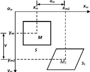
Figure 1.sub-region before and after deformation.
full-field measurements, non-contact, nondestructive to specimen, simple optical path, measurement fields which can be independently adjusted as needed, no interference fringe processing, wide application range, low requirement to environment, simple operation and so on. The pixel was employed by Asundi [11] to measure the displacement of object. Cofaru et al. [12] elaborated on the calculation principles of DIC method, using the method to analyze the test data under low strain rate, and then, obtained the accurate results. High-speed DIC method was applied to three-point bending test which was loaded by Hopkinson bar, and the mechanical properties of aluminum under the action of bending is obtained by Pierron et al. [13]. Kumar et al. [14] applied the DIC method to high strain rate experiment with explosion loading, the bending response of aluminum was measured and agreed well with the simulation results.
Through Taylor impact test, which is a typical plastic dynamic fundamental problem, reverse impact experiments were established. The deformation rules in the Taylor experiments was obtained and simulation was employed to the impact. The reverse ballistic experiment design principles were obtained to act better on the structure response of penetrator. In order to research the plastic wave propagation of specimen in reverse Taylor impact test, DIC was applied to measure the deformation rules of specimens with different velocities and structure, in addition, the plastic wave propagation was analyzed. Then, compared with the simulation results, the deformation of Taylor rod influenced by wave propagation characteristics were further studied, which proves the feasibility of DIC method in reverse ballistic test.
2. Digital image correlation matching
principle
The basic principle of DIC method is matching the geometric point on the digital speckle image of object surface under different status, tracking the movements of point and analyzing the deformation information. Speckles are random distributed in the speckle field, each scattered spots is different with the surrounding point, and the small area surrounding the point is called the sub-region. In the speckle field, a point at the center of sub-region can be used as the displacement carrier, by searching and analyzing
C
Photron SA5 High Speed Camera
energy absorbing bucket
Gus chamber
Computer Inial Velocity
Specimen
Rigid plate
inspecon window light Gun barrel
Target chamber
Figure 2.Reverse Taylor impact experiment layout.
the movement and the change of the sub-region to get the displacement of the point. As shown in Fig. 1, M
is the center point of sub-region S which size ism×m
pixels. When the surface is moving, sub-region S moves to the location of sub-region S1, thus the location of M1 which comes from the feature point M after moving can be obtained and the deformation ofMcan be measured.
Usually a correlation coefficient C will be defined (as shown in formula (1)) to represent the characteristic speckle pattern matching degree of M and M1, its extreme value point shows the best match. DIC matching search algorithm can reach the accuracy of pixel level, but the precision also can’t satisfy the precision of the conventional experimental requirements. Thus, after the pixel level matching, in order to obtain a higher measurement accuracy, special mathematical methods are used to get the position of sub-pixel level matching point. For high quality speckle figure, the measurement precision of DIC displacement can reach 0.01 pixels. The
f (x,y) andg(x∗,y∗) are the pixel matrix ofM andM1, respectively.
C =1−
f (x,y)·g(x∗,y∗)
f2(x,y)·g2(x∗,y∗)1/2· (1)
(a) Launcher system
(b) Target chamber and high-speed camera
(c) Reverse impact specimen in target chamber
Figure 3.Test equipment.
was used to record the experiment process, as shown in Fig. 3(b), shooting frame was 75000 fps, exposure time was 1/424000 s. Because of the high filming frames, two strong illuminants made of tungsten iodine lamps were needed in the target chamber to fill light. For the reverse impact test, the rigid plate was made of 45# steel with a diameter of 48 mm and thickness of 10 mm, which was put into the nylon sabot to launch and polished at the impact end. The specimen was located about 50 cm to the muzzle as shown in Fig.3(c), the gas pressure of the test is 0.6∼1.8 Mpa, impact velocity is 104 m/s∼201 m/s. High- speed camera was used to read the launch velocity, a lot of images were selected before impact to calculate the velocity ranging at pixel level and take average.
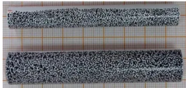
Figure 4.Specimens with speckle in reverse impact test.
Figure 5.D=10 mm specimens’ deformation after impact.
Figure 6.D=15 mm specimens’ deformation after impact.
Because of the use of DIC test system, speckles should be sprayed on the side near to the high-speed camera of the specimens, as shown in Fig. 4, speckles whose size was about 1∼5 pixels need to be sprayed evenly and irregularly. High-speed camera and gas gun were triggered synchronously by trigger device, and the shot pictures can be used for analyzing the structure response of specimens in microsecond level. The propagation speed and mode of plastic wave front can be obtained through the pictures. Then, the strain and displacement distribution diagram can be calculated by DIC method, and the deformation rules of different structure and plastic wave propagation characteristics of specimens were explored.
Figure 7.Finite element models of reverse Taylor impact.
Figure 8. Von Mises stress of No.R9 reverse impact by simulation and specimen after experiment.
No.R10 specimen. The comparison between the thin rods and the thick rods in Fig.5and Fig.6show that the plastic deformation was more easily occurred in thin rods. For the thin rod, when the impact velocity is close to 150 m/s, the barreled region has already appeared. But for the thick rod, the barreled region appeared only when the velocity is above 190 m/s. The appearance of the barreled region explains the plastic wave propagation characteristics in a certain extent.
4. Simulation of reverse Taylor impact
test
In order to further research the reverse Taylor impact, the numerical simulation of Taylor impact was conducted by LS-DANY3D under different working condition and mass ratio.
4.1. Finite element model
The finite element models are shown in Fig.7, because of the symmetry, a quarter model was adopted. For the reverse impact, a solid element and rigid material model was selected for the target which was treated as rigid without deformation. Non-proportional meshing was chosen for the copper specimens, with a dense grid close to the impact end and sparse grid far away. Eroding surface to surface contact was taken between the rod and target during the impact process.
4.2. The contrast between simulation and experiment result
Figure8 shows the von mises stress given by simulation and specimens after experiment of No.R9, and the velocity of No.R9 is 201 m/s. At the beginning of impact, when
t =13µs, the mushroom head was generated. Both the elastic and plastic wave propagated to the far end, but plastic wave velocity is much lower than elastic wave.
Figure 9.Radial strain of No.R10 in the impact process.
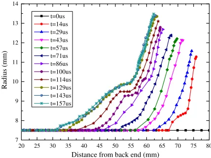
20 25 30 35 40 45 50 55 60 65 70 75 80 7
8 9 10 11 12 13 14
Ra
d
ius (mm
)
Distance from back end (mm) t=0us
t=14us t=29us t=43us t=57us t=71us t=86us t=100us t=114us t=129us t=143us t=157us
Figure 10.The instantaneous outline of No.10.
At t=40µs, the elastic wave arrived at the far end and reflected, the plastic wave still propagated to the far end. Whereafter, the elastic wave bounced and overlapped at back and forth inside the specimen, but the plastic wave propagated in a relatively lower velocity to the far end as before. After t=133µs, obvious movement occurred on reverse impact specimen, the total energy gradually transformed to kinetic energy. Att=173µs, a very weak plastic wave still propagated in reverse impact. As shown in Fig. 8, the deformation in simulation and experiment have a good agreement, which confirms the feasibility of simulation.
5. Results and discussion
Eakins [8] adopted the analysis method similar to Taylor [1], an expression for the stress and strain was derived using the conservation equations of the elastic and elastic/plastic transition fronts. It should be noted that in all cases when conservation laws of mass and momentum are used, the equalities are performed between adjacent time-frames, rather than at a particular instance in time. At the elastic boundary, the rate of mass flow entering the elastic front must be equal to the rate of mass flow leaving the front; hence
d dt(M
i n
)= d
dt(M
out
) (2)
d
dt(ρ0A0Cdt)= d
dt[ρA0(C−Up1)dt] (3)
where Mi n,Mout,A0,ρ
oandρare, respectively, the mass
30 35 40 45 50 55 60 65 70 75 80 0.0 0.1 0.2 0.3 0.4 0.5 0.6 0.7 0.8 Str ain
Distance from back end (mm) t=14us t=29us t=43us t=57us t=71us t=86us t=100us t=114us t=129us t=143us t=157us
Figure 11.The instantaneous strain of No.10.
0 20 40 60 80 100 120 140 160 180 200 0 150 300 450 600 750 900 1050 1200 1350 1500 III II v( m/ s) time(us) Test by DIC program Test by high speed graph Simulation
I
Figure 12.The elastic-plastic interface velocity of No.R10.
conservation of mass to the elastic/plastic transition front, the Eq. (7) gives an equivalent expression for the rate of mass flow when entering and exiting the front
d
dt[ρA0(v−Up1)dt]= d
dt[ρA(v−Up2)dt] (4)
where, v represents the speed when the elastic/plastic transition front (leading plastic wave) moves into elastically strained material, and Ais the increased cross-sectional area just within the plastic zone. Again, the initial area A0 is taken at a position ahead of the elastic/plastic transition front att1, while the strained area Ais taken at that same position after the front has passed at a later time
t2.
Considering the conservation of momentum across the elastic/plastic transition front, by equating the rate of change in momentum to the net impulse. The impulse can be expressed as
Fdt=σ(A0−A)dt (5) where,F is force,σ is stress. Then, the rate of momentum change across the elastic/plastic transition front can be written as
d dt(p
i n−
pout)= d
dt(M
i nvi n−
Moutvout) (6) where, p is momentum, M and v are the mass and corresponding velocity of material entering or exiting the
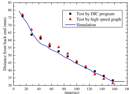
0 20 40 60 80 100 120 140 160 180 30 35 40 45 50 55 60 65 70 75 80 85 Dist ance from b ack end (mm) time(us)
Test by DIC program Test by high speed graph Simulation
Figure 13.The elastic-plastic interface position of No.R10.
0 20 40 60 80 100 120 140 160 180 0 200 400 600 800 1000 1200 1400 P lasti
c wave veloci
ty (
m
/s)
time(µm)
R1, v=135m/s, D=10mm R4, v=154m/s, D=15mm R5, v=147m/s, D=10mm R6, v=104m/s, D=10mm R7, v=116m/s, D=15mm R9, v=201m/s, D=10mm R10, v=193m/s, D=15mm
Figure 14. Time history curve of plastic wave velocity with different impact velocity and structure.
transition front. Considering the density change across the elastic front is negligible, the stress expression can be given by the Eqs. (2)–(6) as
σ =−ρ0A0v2
A =−ρ0v
2(1−ε) (7)
then,
ε= A−A0
A · (8)
Calculation and analysis were conducted on the results of DIC measurement, and the radius strain pictures were obtained. Figure 9 reflects the process of plastic wave propagation in the rod. It can be seen that a tiny vibration was occurred at the beginning of the impact, then the expansion happened at the impact end, and the strain showed a trend of layered. The nearer to the impact side, the greater the strain gradient was. The experiment results are similar to the simulation, which proves the correctness of the above simulation work on the other side.
end, the elastic barreled region rebounded duringt =29∼ 86µs. After t=86µs, the barreled region appeared as a plastic deformation. Then, the deformation gradually slowed down and the impact process ended.
The elastic-plastic interface velocity of No. R10 is shown in Fig.12, considering the theory of Jones et al. [6], the deformation of a Taylor specimen was characterized by three patterns of behavior. The early time behavior, denoted by Phase I, was shock dominated nonlinear motion of the plastic wave front, as shown in Fig.12and Fig.13at 0∼50µs. This was followed by steady motion of the plastic wave front, denoted by Phase II during 50–150µs. This simple description is mostly correct, but it is evident that the velocity of the plastic wave front must come to zero at the end of the event. Hence, a description that includes nonlinear behavior of the wave front at the end of the event is appropriate. This description is represented as the third phase, namely Phase III, in which deceleration of the plastic wave front occurs in 150– 180µs. Notice that the velocity comes to zero at the end of the event. According to the distance from elastic-plastic wave front to impact end in Fig. 13, the trend of wave propagation agree well with the theory of Jones et al. [6], which proves that the DIC method is effective.
Comparing the rods with different impact velocities and different structures during the Taylor impact process, the length of the stable phase of plastic wave propagation is different, but the values of the duration are slightly different. As shown in Fig.14, the stable phase of plastic wave propagation is long when it is at a high impact velocity. For 15 mm diameter rods, the length of stable phase is shorter than that for 10 mm diameter rods, and the propagation velocities are similar. It illustrates that the deformation of 15 mm diameter rods is smaller than that for 10 mm diameter rods.
6. Conclusions
Through reverse Taylor impact tests, the dynamic response data of Taylor rod in microsecond level time resolution was obtained, and the deformation and outlines of the rod at different times were analyzed.
It is better to use the high speed DIC method than traditional optical method to measure the reverse
impact tests. According to the contrast of experiments and simulation, which proved the three stages of plastic wave propagation are basically identical, the propagation characteristic of plastic wave was analyzed. The rules of plastic wave propagation in different rod structures and impact velocities were obtained.
This work was supported by the National Natural Science Foundation of China under Grant (No.11221202) and the National Natural Science Foundation of China (No.11202029, No.11390362).
References
[1] G. Taylor, Proc. R. Soc. London, Ser. A194(1038), 289 (1948).
[2] J. W. House, B. Aref, J. C. Foster, and P. P. Gillis, J. Strain Anal. Eng. Des34(5), 337 (1999).
[3] Davila, J. M. Huntley, G. H. Kaufmann, and D. Kerr, Appl. Opt.44(19), 3954 (2005).
[4] D. C. Erlich and D. A. Shockey, presented at the Shock Waves in Condensed Matter – 1983.American Physical Society Topical Conference, 18–21 July 1983, Amsterdam, Netherlands, 1984 (unpublished). [5] S. E. Jones, P. P. Gillis, J. J. C. Foster, and L. L. Wilson, J. Eng. Mater. Technol 113 (2), 228 (1991).
[6] S. E. Jones, P. J. Maudlin, and J. C. Foster, Int. J. Imp. Eng19(2), 95 (1997).
[7] D. Eakins and N. N. Thadhani, J. Appl. Phys.100(7), 073503 (2006).
[8] D. Eakins and N. N. Thadhani, Int. J. Imp. Eng34 (11), 1821 (2007).
[9] E. Anderson Jr, T. Behner, T. J. Holmquist, and D. L. Orphal, Int. J. Imp. Eng38(11), 892 (2011). [10] E. Lid´en, B. Johansson, and B. Lundberg, Int. J. Imp.
Eng32(10), 1696 (2006).
[11] Asundi, Opt. Lett.25(4), 218 (2000).
[12] Cofaru, W. Philips, and W. Van Paepegem, Meas. Sci. Technol.23(10), 105406 (2012).
[13] F. Pierron, M. A. Sutton, and V. Tiwari, Exp. Mech. 51(4), 537 (2010).