Methodology of using the Adjoint solver optimization tool during
flow in the intercooler filling line to minimize pressure drop
Veronika Horová1, Marian Bojko1,*, and Josef Dobeš2
1Department of Hydromechanics and Hydraulic Equipment, Faculty of Mechanical Engineering, VŠB-Technical University of Ostrava, 17. listopadu 15, Ostrava Poruba, Czech Republic
2Hanon Systems Autopal Services s.r.o., Luzicka 984/14, Novy Jicin, Czech Republic
Abstract. The paper deals with numerical modelling of the flow in the intercooler filling line by Adjoint solver to minimize pressure loss. The ANSYS Fluent software was used for the calculations. The basic flow calculation was performed in the first phase. Then the mathematical model with Adjoint solver optimization tool was defined. The numerical calculation was unstable and did not lead to a convergent solution, because of creation of vortexes. The mathematical model was simplified in the second phase. To suppress instabilities and vortices a dynamic viscosity of coolant was adjusted. The pressure gradients between inlet and outlet for unmodified geometry and for modified geometry were evaluated. The final evaluations of pressure drop changes were implemented for modified geometry with original dynamic viscosity of the coolant.
1 Introduction
The optimization of a design using numerical flow modelling is an important part of the designing process and following manufacturing process. This make unnecessary to create physical models for practical exploring. This saves time and especially saves finances. It is necessary to create and define a suitable 3D model for optimization. The 3D model is solved numerically to obtain the necessary data. There are many optimization methods. The best known optimization method is the gradient-based method that works with a large number of design variables. The gradient-based method uses computational schemes such as finite difference scheme and adjoint scheme to solve. The adjoint method is more preferable because it is independent on the design variables and performs the calculation only once. This method is part of the ANSYS Fluent software (Adjoint Solver), which allows to get information about the sensitivity of a fluid system that is difficult to get in another way. The Adjoint Solver extends the analysis that is contained in the standard flow solver. The user must complete all necessary information when simulating using a standard flow solver. The information includes mesh, materials properties, physical model and boundary conditions. If the flow calculation converges, the standard solver will provide a dataset describing the flow. The application of the Adjoint Solver in ANSYS Fluent software is the content of the publications [1, 2]. There is described the methodology of application of the optimization tool on the examples of flow in a duct in car climate system and in a flow passage of the check valve.
This paper describes the methodology of using Adjoint Solver applied on the intercooler entry connector used in the automotive industry.
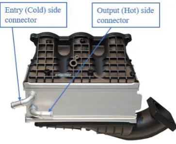
The intercooler (Figure 1) is a technical device that serves to heat exchange in supercharged automobile engines. The filling line is used to connect the pressure energy source with the cooling plates.
Fig. 1. Water charge air cooler
The use of the Adjoint Solver is unstable in applications where there are vortices or other instabilities in the flow field, which are created as a result of flow separation. This Adjoint Solver instability characteristic presents the issue of the solution for the intercooler entry connector that is content of this paper.
To prevent creating vortices, the dynamic viscosity of the coolant was adjusted. This change has led to convergent solution.
Currently, there is an increase in operating design parameters, which may be associated with the occurrence of cavitation [3] in certain geometry areas, such as narrowing. The use of the Adjoint Solver can predict these areas by evaluating pressure field.
2 Mathematical model characteristics
The mathematical model is defined by balance equations which describes the flow. They are continuity equation, Navier-Stokes equations, energy equation and more [4, 5]. During the flow calculation on the entry connector geometry the energy equation was not used because the isothermal flow was defined.
There are several mathematical models of turbulence available in ANSYS Fluent software. The most used mathematical models of turbulence include dual-equation
k-ε mathematical model and k-ω mathematical model. There are three major modifications for the k-ε
mathematical model of turbulence. They are k-ε Standard,
k-ε RNG a k-ε Realizable [4]. The k-ε RNG mathematical model of turbulence is suitable for lower Reynolds numbers in existence of vortices and secondary flow. Reynold’s critical number indicates the transition between the laminar and the turbulent flow and is defined by:
𝑅𝑒 =𝑣 ∙ 𝑑
𝜐 (1)
v…velocity [m.s-1]
d…hydraulic diameter [m]
υ…kinematic viscosity [m2.s-1]
Dynamic viscosity is defined by:
𝜂 = 𝜐 ∙ 𝜌 (2)
υ…kinematic viscosity [m2.s-1]
ρ…density [kg.m-3]
Changing the dynamic viscosity reduced the Reynolds number and the flow regime was changed to laminar.
Adjoint Solver
Adjoint Solver [6] in ANSYS Fluent software is a tool that allows you to get information about the sensitivity of a fluid system that is difficult to get in another way. The Adjoint Solver performs a calculation that is very similar to the standard calculation. The difference is that scalar
observation is selected before the calculation starts. If the convergence of the adjoint solution occurs, we obtain derivations of the observe magnitude relative to the position of each individual point located on the surface of the geometry. This determines the sensitivity of the monitored variable for a particular boundary condition setting. The final calculation of the adjoint task can be used as a pattern for the design change.
ANSYS Fluent software includes a discrete adjoint solver. By using a discrete adjoint solver, we get information for various problems, including the wall functions problem. The use of Adjoint Solver may be unstable, especially in applications where there are vortices or other instabilities in the flow field. Adjoint Solver stability can be problematic at high Reynolds numbers, especially when dealing with large numbers of cells and complex geometry. To overcome these problems, two stabilization schemes are available in ANSYS Fluent software (Spatial Scheme and Modal Scheme) [7].
Mesh, Boundary conditions, Physical properties
The mesh was created in the ANSYS Meshing. The mesh was densified near the wall according to the wall function. The suitability of the wall function was verified by evaluating the progress of parameter y+ [3] with additional adaptation. The result was a mesh with 4206535 elements.
The mathematical model characteristic is presented in Table 1. In Table 2 there are boundary conditions which were defined. In Table 3 there are physical properties of the coolant at 35°C.
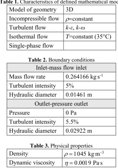
Table 1. Characteristics of defined mathematical model Model of geometry 3D
Incompressible flow constant Turbulent flow k-ε, k-ω
Isothermal flow T=constant (35°C) Single-phase flow
Table 2. Boundary conditions Inlet-mass flow inlet Mass flow rate 0.264166 kg.s-1 Turbulent intensity 5%
Hydraulic diameter 0.01461 m Outlet-pressure outlet
Pressure 0 Pa
Turbulent intensity 5.5% Hydraulic diameter 0.02922 m
Table 3. Physical properties Density kgm Dynamic viscosity .Pas
viscosity was adjusted to 1 Pa.s to ensure a stable and convergent calculation of adjoint variables. By adjusting the dynamic viscosity, the Reynold’s number was reduced and more uniform flow character can be assumed. With respect to reduction of Reynold’s number a k-ε RNG with Enhanced Wall Treatment mathematical model of turbulence was used. This mathematical model of turbulence is suitable for lower Reynold’s numbers.
3
Mathematical model application-basic
flow
The basic flow was calculated in the first phase. The coolant was water-glycol in ratio 60/40 (60 % water, 40 % glycol). Several mathematical models of turbulence have been tested. It was used k-ε RNG with Enhanced Wall Treatment mathematical model of turbulence for evaluation, which is suitable for lower Reynolds numbers.
The progress of parameter y+ was evaluated. The value of a parameter y+ was about 1 which means that the wall function was appropriately selected. The calculation was applied to the entry connector geometry (Figure 2). Figure 2 shows the entry and output connector to intercooler. Inlet and outlet boundary conditions are marked here.
Fig. 2. Entry and output connector
In Figure 3 there is a comparison of the pressure drop values between inlet and outlet (ΔpIN,OUT = ΔpIN - ΔpOUT)
for several mathematical models of turbulence.
Fig. 3. Comparison of mathematical models of turbulence
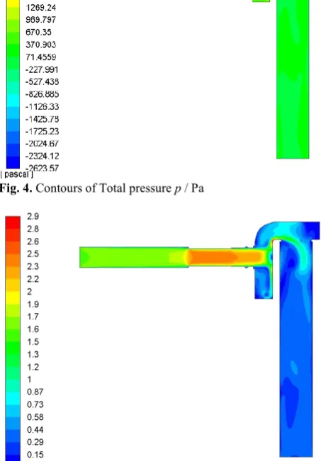
The contours of total pressure (Figure 4) and contours of velocity magnitude (Figure 5) were evaluated in the longitudinal section of the computing area.
Fig. 4. Contours of Total pressure p / Pa
Fig. 5. Contours of Velocity Magnitude v / m/s
4 Adjoint Solver application
Fig. 6. Divergent residuals
There are several options to achieve convergent solution e.g. switch to a time-dependent solution, which Adjoint Solver does not allow. The dynamic viscosity of coolant was adjusted to 1 Pa.s to avoid formation of vortices. By adjusting the dynamic viscosity, a more uniform flow character can be assumed. This provides stable and convergent calculation of adjoint variables. Then the optimization was performed. Any stabilization scheme was used during the calculation of adjoint variables.
The procedure of performing the shape optimization in the Adjoint Solver in individual steps is described in the next chapter.
Optimization methodology
The deformation region was defined only on the inlet part of the entry connector as shown in Figure 7.
Shape optimization steps:
• Pressure drop ΔpIN,OUT evaluation
• Shape Sensitivity Magnitude evaluation • Pressure drop expected change evaluation • Modification of geometry
• Contours of Normal Optimal Displacement evaluation • Display geometry change result
• The basic flow calculation • The adjoint variables calculation
The pressure drop between inlet and outlet ΔpIN,OUT for
unmodified geometry was evaluated in the first step. Then the Shape Sensitivity Magnitude was evaluated (Figure 7), which is a prediction before the optimization of the geometry. It displays areas where the pressure drop is most sensitive to shape of geometry.
Fig. 7. Shape Sensitivity Magnitude
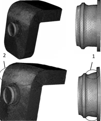
The result of deformation of the computing area was evaluated in the next step. The unmodified and modified geometry were compared. A Figure 8 shows deformed areas. As show a Figure 8 the input part of the connector tends to expand (detail 1), and slight rounding also occurs on the upper surface of the connector body (detail 2).
Fig. 8. Deformation: unmodified geometry (Top), modified geometry (Bottom)
A calculation of the basic flow field on the modified geometry was performed and a pressure drop between inlet and outlet (ΔpIN,OUT = ΔpIN - ΔpOUT) was evaluated.
There were 5 optimizations performed. In the Table 4 there is a comparison of ΔpIN,OUT between original
geometry and geometry after optimization.
Table 4. Evaluation of ΔpIN,OUT(η=1 Pa.s), percentage decrease
ΔpIN,OUT [Pa]
Unmodified geometry 46719.45
Modified geometry 45003.41
Decrease [% ] 3.67
As can be seen from the Table 4, the pressure drop between inlet and outlet for a changed dynamic viscosity dropped by 3.67 %.
In the last step, a calculation of the basic flow field for the modified geometry was performed. The dynamic viscosity was defined to the original value (0.0019 Pa.s).
The pressure drop between inlet and outlet ΔpIN,OUT
was evaluated again and compared with ΔpIN,OUT for the
original unmodified geometry.
Table. 5. Evaluation of ΔpIN,OUT(η=0.0019 Pa.s), percentage
decrease
ΔpIN,OUT [Pa]
Unmodified geometry 3186.6
Modified geometry 2425.3
Decrease [% ] 23.9
The pressure drop between inlet and outlet after a recalculation with the original viscosity dropped by 23.9 %, as shown in the Table 5.
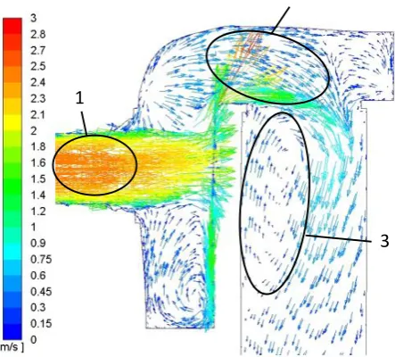
The character of the flow field was evaluated by a vector field in longitudinal section of the computing area with original viscosity (0.0019 Pa.s) for unmodified geometry (Figure 9) and for modified geometry (Figure 10).
Fig. 9. Velocity Vectors Colored by Velocity Magnitude v / m/s: unmodified geometry
Fig. 10. Velocity Vectors Colored by Velocity Magnitude v / m/s: modified geometry
The vector fields for both variants were evaluated in the same range. It is obvious a higher maximum speed in the inlet mid-section (detail 1), as shown in Figure 10. There is a decrease in speed (detail 2) in the transition section of the outlet pipe. There is also a different type of vortex in the output pipe. The vortex is extended more to the wall (detail 3).
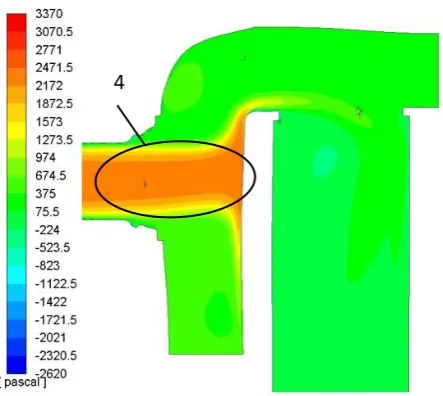
The contours of total pressure for unmodified geometry (Figure 11) and for modified geometry (Figure 12) with the original viscosity in the longitudinal section of the computing area were evaluated. These both variants were evaluated in the same range. The modification will reduce the total pressure in the input part of the computing area (detail 4) compared to the unmodified geometry (Figure 11).
An analogous result with the vector field is apparent. The velocity has increased in this area, i.e. the total pressure drops. This result is also evident by the pressure drop ΔpIN,OUT evaluation.
Fig. 11. Contours of Total Pressure p / Pa: unmodified geometry
1
2
Fig. 12. Contours of Total Pressure p / Pa: modified geometry
5 Conclusion
This paper deals with the methodology of using the Adjoint Solver optimization tool to minimize pressure drop in ANSYS Fluent software. The basic flow was calculated on the intercooler entry (cold) connector geometry in the first phase. The coolant was water-glycol in ratio 60/40. Several mathematical models of turbulence have been tested. It was used k-ε RNG Enhanced Wall Treatment mathematical model of turbulence for evaluation. By evaluating parameter y+ was verified that this mathematical model of turbulence is used correctly.
The shape optimization in Adjoint Solver was performed on the entry (cold) connector geometry (Figure 2). There are vortexes in the computing area and neither the use of stabilization schemes has not led to a convergent solution (Figure 6). The dynamic viscosity of coolant was adjusted to 1 Pa.s to avoid formation of vortices. This provides stable and convergent calculation of adjoint variables. Then the optimization was performed. The deformation region was defined only on the inlet part of the entry connector as shown in Figure 7. The optimization was performed according to a mentioned methodology. The result of deformation of the computing area was evaluated in the next step. As show a Figure 8 the input part of the connector tends to expand, and slight rounding also occurs on the upper surface of the connector body.
A calculation of the basic flow field on the modified geometry was performed with changed dynamic viscosity (η=1 Pa.s) and a pressure drop between inlet and outlet
ΔpIN,OUT was evaluated. As can be seen from the Table 4,
the pressure drop between inlet and outlet for the changed dynamic viscosity dropped by 3.67 %. In the last step, a calculation of the basic flow field for the modified geometry was performed. The dynamic viscosity was defined to the original value (0.0019 Pa.s). The pressure drop between inlet and outlet ΔpIN,OUT was evaluated
again. The pressure drop between inlet and outlet after a recalculation with the original viscosity dropped by 23.9 %, as shown in the Table 5.
This paper was supported by the Project No. CZ.02.1.01/0.0/0.0/16_019/0000867 „European Regional Development Fund in the Research Centre of Advanced Mechatronic Systems project” within the Operational Programme Research, Development and Education.
References
1. A. Tzanakis, Duct optimization using CFD software ´ANSYS Fluent Adjoint Solver'. Chalmers University of Technology in Göteborg, pp. 42, (2014)
2. M. Kozubková, M. Bojko, L. Hružík, 37th Meeting of Departments of Fluid Mechanics and Thermodynamics, Investigation of flow for check valves using the optimization method, 2000 (2018). 3. R. Sikora, A. Bureček, L. Hružík, M. Vašina, EPJ
Web of Conferences, EFM14 Experimental investigation of cavitation in pump inlet, 92, 02081, (2015)
4. M. Kozubková, Modelování proudění tekutin: FLUENT, CFX , VŠB-TUO, pp. 153, (2008) 5. M. Kozubková, T. Blejchař, M. Bojko, Modelování
přenosu tepla, hmoty a hybnosti,VŠB-TUO,pp. 174, (2011)
6. ANSYS FLUENT Manual. ANSYS FLUENT Advanced Add-On Modules Version 16.2. ANSYS, Inc., pp. 474, (2015)
7. M. Kozubková, M. Bojko, Aplikace adjungovaného řešiče teorie, VŠB-TUO, (2015)