R E S E A R C H
Open Access
Multi-antenna transmission for underlay and
overlay cognitive radio with explicit
message-learning phase
Ricardo Blasco-Serrano
1*, Jing Lv
2, Ragnar Thobaben
1, Eduard Jorswieck
2and Mikael Skoglund
1Abstract
We consider the coexistence of a multiple-input multiple-output secondary system with a multiple-input
single-output primary link with different degrees of coordination between the systems. First, for the uncoordinated underlay cognitive radio scenario, we fully characterize the optimal parameters that maximize the secondary rate subject to a primary rate constraint for a transmission strategy that combines rate splitting and interference cancellation. Second, we establish a model for the coordinated overlay cognitive radio scenario that consists of a message-learning phase followed by a communication phase. We then propose a transmission strategy that combines techniques for cooperative communication and for the classical cognitive radio channel. We optimize our system to maximize the rate of communication for the secondary users under a primary-user rate constraint and find efficient algorithms to compute the optimal system parameters. Finally, we compare both cognitive radio strategies to assess their relative merits and to evaluate the effect of the message-learning phase. We observe that for closely located transmitters, the overlay strategy outperforms the underlay strategy. In this situation, learning the primary message is very beneficial for the secondary systems, especially if they are interference-limited rather than power-limited. The situation is reversed when the distance between the transmitters is large. In either case, we observe that there is room for significant improvement if the transmitter implements both strategies and decides adaptively which one to use according to the channel conditions. We conclude our work with a discussion on the extension to the coexistence with multiple-input multiple-output primaries.
Keywords: Cognitive radio; Underlay; Overlay; Multiple antennas; Message learning; Cooperation
1 Introduction
The scarcity of available spectrum for accommodating new services in combination with the underutilization of currently allocated spectrum has fueled research on alter-native visions on communications over the last decade. It has been suggested that new, unlicensed (i.e. secondary) users could utilize portions of the spectrum licensed to primary users as long as the latter are not significantly affected. In this context, the concept of cognitive radio, with its promise of reconfigurability and adaptability to varying conditions, has emerged as a strong candidate for
*Correspondence: [email protected]
1ACCESS Linnaeus Centre, School of Electrical Engineering, KTH Royal Institute of Technology, Stockholm, Sweden
Full list of author information is available at the end of the article
implementing communication systems that make a more efficient use of the spectrum.
Three major cognitive radio paradigms that consider different degrees of interaction between primary and sec-ondary users have been identified: interweave, underlay and overlay [1,2]. Interweave cognitive radio is concep-tually the simplest one: the secondary devices sense the environment to detect the presence of primary users and transmit opportunistically only when these are silent. Underlay cognitive radio goes one step further and per-mits communication between secondary users as long as the disturbance created to the primary system is below some predefined threshold. Clearly, in this case, the sec-ondary terminals need not only assess whether primary users are transmitting or not but also how much inter-ference they will create and whether this will disrupt the primary communication. Finally, the overlay paradigm
allows for a tight interaction between primary and sec-ondary systems. Of course, this comes not only at the price of a higher degree of sophistication of the secondary terminals but also requires flexibility in the primary sys-tem. Nevertheless, in all three cases, it is necessary to assess the impact of the presence of secondary users on primary systems. Several measures have been discussed in the literature for this purpose, for example, the proba-bilities of miss detection and interference for interweave cognitive radio or, more in general, soft- and peak-power-shaping interference temperature constraints [3,4]. An alternative is to consider directly the degradation suffered by the primary users, for example, in terms of the loss in rate [5].
Research on the physical layer has focused on estab-lishing basic models for the different cognitive radio scenarios, deriving their fundamental limits, and design-ing practical transceivers that come close to these limits. From an information theoretic point of view, two chan-nel models have been considered for the three cogni-tive radio paradigms: the Gaussian interference channel [6,7] and the cognitive radio channel [8-10]. As described before, in the cases of interweave and underlay cognitive radio, there is no cooperation between primary and sec-ondary systems. This is precisely the situation described by the interference channel. The interweave cognitive radio paradigm corresponds to time sharing in the inter-ference channel [6], with a sharing parameter that is fixed by the activity of the primary users. In this case, the challenge lies almost exclusively in sensing accurately the primary activity, a topic that lies outside the scope of this paper (see, e.g. [11] and references therein). Therefore, interweave cognitive radio scenarios will not be consid-ered here. On the other hand, in the case of underlay cognitive radio, primary and secondary systems can trans-mit at the same time and thus the scenario is richer from the point of view of the communication strate-gies that can be used. This is well characterized by the interference channel if one places some additional restric-tions on the model. For example, one usually restricts the communication strategies used by the primary user pairs to consist of point-to-point codes and single-user decoding.
In contrast, overlay cognitive radio scenarios are not described properly by the interference channel. The main reason for this is that the interference channel does not allow for any active cooperation between the user pairs. With the aim of overcoming this limitation, the cogni-tive radio channel was introduced in [9]. This model extends the interference channel by assuming that the secondary transmitter has non-causal knowledge of the primary message. This additional knowledge allows for asymmetric cooperation in the sense that the secondary transmitter can help the primary users to carry their
communication. In addition, it can combat the interfer-ence that the primary signal creates on the secondary receiver by means of interference cancellation or dirty-paper coding. This asymmetric cooperation was key for establishing the capacity of the cognitive radio channel with weak interference [8,9].
A usual system design criterion is to maximize the rate of transmission for the secondary users while ensuring a minimum quality of service (QoS) for the primary users. A key observation is that multiple trans-mit antenna techniques are a powerful and efficient way of controlling the disturbance created by the secondary users [12]. Unfortunately, the use of such techniques often leads to complex matrix optimization problems. This has motivated the use of tools from optimiza-tion theory for the design of transceivers. For exam-ple, convex optimization tools were used in [13] to study underlay cognitive radio models with single-user decoders. An underlay scenario with rate splitting and multiple-user decoding was considered in [14]. The prob-lem of distributed beamforming and rate allocation in decentralized cognitive radio networks was treated in [15]. In a more general framework, the set of effi-cient strategies for multiple-input single-output (MISO) interference networks was characterized in [16,17] in terms of beamformers. The extension of the cog-nitive radio channel to the input multiple-output (MIMO) case was introduced in [18]. Overlay cognitive radio strategies for this channel with par-tial channel state information were considered in [19]. Optimal beamforming for the coexistence of a MIMO secondary user with a MISO primary user with non-causal knowledge of the primary message was consid-ered in [20]. We studied the coexistence of a MISO secondary system with a single-input single-output pri-mary system in [21] for different levels of channel state information, and considered linear precoding strategies in [22].
primaries finish their transmission earlier or to exploit the inefficiencies of the ARQ protocol [23,24]. Similarly, in [25], the secondary system acquires the primary mes-sage and uses it to help the primary system finish the transmission earlier and then use the channel during the idle period. However, these schemes do not fully exploit the possibilities of overlay cognitive radio, in particu-lar the possibility of interaction between primary and secondary systems. The use cooperative communication techniques [26-28] as an enabling technology for cog-nitive radio networks was surveyed in [29]. They were considered in [30] for single-antenna overlay cognitive radio and evaluated in terms of outage probabilities. The optimal secondary power allocation and phase split in a two-phase spectrum sharing scenario was consid-ered in [31]. In [32], the authors studied beamforming and power allocation for the coexistence of a primary single-input single-output (SISO) user with a secondary single-input multiple-output or MISO that acquired the message in a causal fashion. However, as opposed to the work presented here, their work focused only on the second phase of communication, without consider-ing explicitly the first, learnconsider-ing phase. In [33], beam-forming and power allocation were studied for a system, where the secondary users relay the primary signal in an amplify-and-forward fashion, and the performance of the proposed system was compared to an underlay cognitive radio scheme. The use of cooperative relaying mechanisms for spectrum sensing and secondary user transmission in cognitive radio systems was described in [34,35].
1.1 Contributions and outline
We study physical-layer aspects of cognitive radio com-munications in a scenario, where a MISO primary sys-tem coexists with a half-duplex MIMO secondary syssys-tem. We consider two approaches: on one hand, an underlay cognitive radio model without any cooperation between primary and secondary systems. On the other hand, an overlay cognitive radio model that allows for causal coop-eration between the systems. Our goal is to compare both strategies and assess the potential advantages of each of them under conditions that are more realistic than the original cognitive radio channel model in [8,9]. In par-ticular, we require that the primary message be learned causally by the secondary system.
We emphasize that this paper deals with idealized mod-els. In particular, the overlay scenario requires a high degree of cooperation between primary and secondary systems. Similarly, quite often, the terminals have access to larger portion of channel state information than in practical systems. In spite of this idealization, we have decided to take this approach to quantify the benefits of having coordinated primary and secondary system
(through the message-learning phase) in a quite general way, as compared to the moread hocapproaches in [23-25]. Moreover, these systems are, at least in theory, imple-mentable, unlike the less realistic scenarios where the secondaries have non-causal knowledge of the primary messages.
This paper extends our previous work on the coexis-tence of a SISO primary system with a MISO secondary link for underlay [14] and overlay systems [36] to the case of coexisting MISO primary and MIMO secondary sys-tems. The addition of multiple antennas at the primary transmitter and secondary receiver results in a model that is richer and substantially more complex. In particular, for the overlay scenario, the new model allows not only for MIMO communication between secondary users but also for MIMO inter-transmitter communication. Moreover, this new channel configuration represents a departure from the interference network (e.g. [17]) as it also incorpo-rates aspects from cooperative communications. Finally, note that the convex optimization framework developed in [13] for underlay cognitive radio is not directly applica-ble to the strategies presented here because they result in non-convex problems.
2 Preliminaries 2.1 Notation
Column vectors and matrices are represented in lower case and upper case boldface letters, respectively. |·| is the absolute value of a scalar or the determinant of a matrix,·is the Frobenius norm of a vector or matrix, and(·)H stands for Hermitian transpose. The trace of a square matrix is denoted by tr{·}.X X
XHX−1XH
denotes the orthogonal projection operator onto the col-umn space ofX, and⊥X I−X, whereIis the identity matrix, denotes the orthogonal projection operator onto the orthogonal complement of the column space of X. The notationX 0 denotes that the matrixXis positive semidefinite. All logarithms in this paper are taken to the base of 2, and all rates are expressed in bits.
2.2 System model
We consider a MISO primary system withNT,1transmit antennas that is willing to share its channel with a half-duplex MIMO secondary system withNT,2antennas at the transmitter andNR,2antennas at the receiver. Our goal is to compare basic communication strategies for underlay and overlay cognitive radio without assuming non-causal knowledge of the primary message at the secondary trans-mitter. For this purpose, we introduce the following two channel models.
2.2.1 Underlay cognitive radio
We use the Gaussian MIMO/MISO interference chan-nel as a model to study the conflict between a primary and a secondary link in underlay cognitive radio. Each of the transmitters sends a signal that is observed by the intended receiver in the presence of interference (from the other transmitter) as well as white Gaussian noise. The tth received sample from the matched-filtered complex baseband model is
y1(t)=hH11x1(t)+hH21x2(t)+n1(t) (1)
y2(t)=HH12x1(t)+HH22x2(t)+n2(t), (2)
wherex1(t)andx2(t)are theNT,1×1 andNT,2×1 signal vectors sent by the primary and secondary transmitters, respectively,hi1is theNT,i×1 vector of the channel gains from transmitter i ∈ {1, 2}to receiver 1, and Hi2 is the
NT,i×NR,2matrix of channel gains from transmitter i ∈ {1, 2}to receiver 2. The scalary1(t)and the vectory2(t) are the observations at the receivers, which are corrupted by the noise processesn1(t)andn2(t), respectively.
2.2.2 Overlay cognitive radio
Our model for communication with half-duplex devices in an overlay cognitive radio environment is illustrated in Figure 1 and consists of two phases. In the first phase, the primary transmitter broadcasts its message to both its intended receiver and the secondary transmitter. The tth received sample from the matched-filtered complex baseband model in this phase is
y1(1)(t)=hH11x1(1)(t)+n(11)(t) (3)
yst(t)=HHt x1(1)(t)+nst(t), (4) where x(11)(t) is the NT,1× 1 signal vector sent by the primary transmitter,h11 is theNT,1×1 vector of chan-nel coefficients between primary transmitter and receiver, and Ht is the NT,1 × NT,2 matrix of channel coeffi-cients between both transmitters. The scalar y(11)(t)and the NT,2 × 1 vector yst(t) are the observations at the primary receiver and secondary transmitter, respectively, which are corrupted by the noise processes n(11)(t) and
nst(t), respectively. Note that, in principle, the secondary receiver can also obtain its own observationy(21) of the primary signal. However, as we shall see, this does not pro-vide any gain for the transmission strategy proposed in Section 4.1.
The second phase corresponds to the set-up which is known as the cognitive radio channel. In this phase, the secondary transmitter can make use of the knowledge of the primary message (obtained in a causal fashion in the first phase). The model in this phase is
y(12)(t)=hH11x(12)(t)+hH21x(22)(t)+n(12)(t) (5)
y(22)(t)=HH12x(12)(t)+HH22x(22)(t)+n2(t), (6) wherex(12)(t)andx2(2)(t)are theNT,1×1 andNT,2×1 signal vectors sent by the primary and secondary transmitters, respectively,hi1is theNT,i×1 vector of channel gains from transmitter i ∈ {1, 2}to receiver 1, andHi2is theNT,i× NR,2matrix of channel gains from transmitter i∈ {1, 2}to
receiver 2. The scalary(12)(t)and the vectory(22)(t)are the observations at the receivers, which are corrupted by the noise processesn(12)(t)andn2(t), respectively.
The entire transmission is carried out overn channel uses;kchannel uses are consumed during the first trans-mission phase, and(n−k)channel uses during the second phase. The fraction of the channel uses in the first and the second phases is given byα=k/nand 1−α, respectively. We will assume that the channels remain constant during the duration of the two phases.
Noise and channel statistics For both underlay and overlay cognitive radio models, the noises at the receivers are modeled by independent circularly symmetric addi-tive white Gaussian noise processes with unit variance: n1,n(11),n(12) ∼CN(0, 1),n2,nst∼CN(0,I). In this paper, we assume that all nodes have perfect channel knowl-edge on all links. In order to evaluate the average behavior of our transmission strategies for different realizations of the channel coefficients, we will model the entries of
Ht,h11,H12,h21, andH22 as samples from independent circularly symmetric Gaussian processes with zero mean with appropriate variances.
3 Underlay cognitive radio
In this section, we introduce the transmission strategy that we consider for the underlay cognitive radio paradigm. Our goal is to maximize the communication rate of the secondary users while ensuring that the primary users have a minimum QoS, defined in terms of a minimum rateR1.
3.1 Underlay transmission strategy
We consider the extension to MIMO secondary systems of the underlay transmission strategy introduced in [14]. The primary transmitter is oblivious to the presence of the sec-ondary users and broadcasts its single-stream signal with powerP1using the covariance matrixK1corresponding to the maximum-ratio transmit (MRT) beamformer, i.e.
K1 = P1h11h
H
11
h112. The primary receiver decodes the mes-sage in the presence of interference from the secondary system and noise. The secondary transmitter splits its message into two parts (i.e. rate splitting) using possi-bly different covariance matrices with possipossi-bly different powers for each of the parts:K2,1andK2,2, respectively. The secondary receiver performs successive/interference decoding to recover the first part of the secondary mes-sage, then the primary message (i.e. the interference), and finally the second part of the secondary message.
The communication rate for the primary users is
Rund1 log
1+ h
H
11K1h11 1+hH21(K2,1+K2,2)h21
, (7)
and the rate achieved by the secondary users is
Rund2 logI+H
H
22(K2,1+K2,2)H22+HH12K1H12 I+HH22K2,2H22+HH12K1H12 +logI+HH22K2,2H22. (8)
The first term in (8) corresponds to the part of the sec-ondary message decoded in the presence of interference (both from primary transmitter and self-interference). The second term in (8) corresponds to the part of the sec-ondary message recovered after decoding and subtracting the primary message. This adds the constraint that the secondary receiver must be able to decode the primary message as well. That is,
Rund1,2 logI+H
H
22K2,2H22+HH12K1H12 I+HH22K2,2H22
. (9)
In addition, we have the constraint on the QoS for the primary user, i.e.Rund1 ≥ R1. Note that by setting appro-priatelyK2,1andK2,2, we obtain the extreme cases, where the secondary receiver decodes first the primary message or does not decode it at all.
We remark that we do not make any assumption on the rank of the matrices K2,1 or K2,2. Basic consid-erations on the number of transmit/receive antennas required for multiple-stream transmission apply here, too (see e.g. [37]).
3.2 Problem formulation
The problem of finding the covariance matricesK2,1and
K2,2 that maximize the secondary rate under the afore-mentioned constraints is expressed as
max K2,1,K2,2
Rund2 (10a)
subject to:
Rund1 ≥R1, (10b)
Rund1,2 ≥R1, (10c)
tr{K2,1+K2,2} ≤P2, (10d)
K2,10,K2,20, (10e)
where it is implicitly assumed that (10c) applies only if
K22 = 0. Note that this problem is not concave due to the constraints (10b) and (10c). Constraint (10b) can easily be transformed into a linear constraint. However, dealing with (10c) is more involved.
3.3 Optimal transmission parameters
The following proposition characterizes the solution to (10). This extends the result in [14] to MIMO secondaries.
Case 1: If
R1≥logI+HH12K1H12, (11)
then decoding the primary message at the sec-ondary receiver is not possible at all. Without interference decoding, we have thatK2,2=0, and
K2,1is the covariance matrix that maximizes
logI+H
H
22K2,1H22+HH12K1H12 I+HH12K1H12
(12)
subject to the corresponding constraints. This is equivalent to solving the following concave prob-lem:
max
log
I+HH22H22+HH12K1H12 (13a)
subject to:
tr{hH21h21} ≤Pintund, (13b)
tr{} ≤P2, (13c)
0, (13d)
where
Pundint h
H
11K1h11 2R1−1 −
1. (14)
Case 2: If
R1≤logI+H
H
22H22+HH12K1H12 I+HH
22H22 ,
(15)
whereis the covariance matrix that solves the concave problem
max
log
I+HH22H22 (16a)
subject to:
tr{hH21h21} ≤Pintund, (16b)
tr{} ≤P2, (16c)
0, (16d)
with Pundint as defined in (14), then it is possible to decode the interference directly, without using rate splitting. Thus, the optimal covariance matrices areK2,1=0andK2,2=.
Case 3: In all other cases, i.e. if
logI+H
H
22H22+HH12K1H12 I+HH22H22
<R1<logI+HH12K1H12, (17) the problem is solved byK2,1= γandK2,2 = (1−γ ), where γ ∈[ 0, 1] is chosen such that Rund1,2 = R
1, and is the matrix that solves the
following concave problem
max
I+H
H
22H22+HH12K1H12 (18a)
subject to:
tr{hH21h21} ≤Pundint , (18b)
tr{} ≤P2, (18c)
0, (18d)
with Pundint as defined in(14).
Proof. The proof is provided in Appendix 1.
Remark 1. In all three cases, the solution can be effi-ciently obtained using convex optimization tools [38].
Remark 2. The preceding results for case 3 reveal that the same covariance matrix (up to a scaling factor) is used for both parts of the secondary message when using rate splitting. For the case of beamformers, which are optimal for MISO secondaries (see e.g. [17] or [39]), this means that it suffices to consider the same beamformer for both parts of the secondary message (cf. [14]).
4 Overlay cognitive radio with explicit message-learning phase
In this section, we introduce the transmission strategy that we consider for the overlay cognitive radio paradigm. Our goal is again to maximize the communication rate of the secondary users while ensuring that the primary users have a minimum QoS, defined in terms of a minimum rateR1.
4.1 Overlay transmission strategy
Our strategy for overlay cognitive radio combines coop-erative communication techniques, in particular decode-and-forward (DF) [26-28], with communication for cognitive radio channels [8,9]. The strategy makes full use of the potential of overlay cognitive radio by estab-lishing active asymmetric cooperation between the users. The protocol establishes transmission of the primary mes-sage in two phases. Moreover, the primary transmitter chooses the system parameters as to maximize the sys-tem efficiency while ensuring that its message is reliably communicated. The secondary transmitter, which only broadcasts during the second phase, not only sends its own message but also acts as a relay for the message of the primary users. In addition to this, some degree of coop-eration in the process of channel estimation is required so that the transmitters obtain the relevant channel state information.
broadcasts its message using theNT,1antennas with trans-mit covariance matrix K(11) 0. The primary receiver and secondary transmitter listen to this transmission. Consider the rates
R(11)αlog
1+hH11K(11)h11
, (19)
RtαlogI+HHt K
(1)
1 Ht, (20)
and letP(11)denote the power spent by the primary trans-mitter in the first phase, i.e.P(11) tr{K(11)}. Expressions (19) and (20) correspond to the rates from the primary transmitter to the primary receiver and to the secondary transmitter in the first phase, respectively.
If the channel Ht is significantly better than h11 (e.g. tr{HHt Ht} h112), then the secondary transmitter will need less redundancy to decode the message. In particular, if
R(11)<R1≤Rt, (21)
then the secondary transmitter can decode the primary message but the primary receiver cannot. Although it cannot decode, the primary receiver has collected use-ful observations of the primary signal. Roughly speaking, it only needs additional redundancy to resolve its uncer-tainty and be able to decode [26].
Once the secondary transmitter is able to decode, the system can switch to the second phase. The second phase has the duration 1− α and consists of two simultane-ous transmissions. On one hand, primary and secondary transmitters cooperate to resolve the uncertainty of the primary receiver. They act as one single virtual transmitter that uses a virtual covariance matrix
Kco= K
(2)
1
H 1−1αKr
(22)
to send the remaining part of the primary message over the extended channelhHext=[hH11,hH21] that consists of the concatenation of both channels to the primary receiver. The sub-matricesK(12) andKr correspond to actual the covariance matrices used by each transmitter, while the sub-matrix corresponds to correlation of the signals sent by each transmitter, so that they add constructively at the receiver (cf. [18], Eq. (3)). Note that while they act coordinately, each transmitter has an independent power constraint (i.e. on tr{K(12)} and tr{Kr}, respec-tively): the primary transmitter uses the power left after the first phase, while the secondary uses only a fraction
of its available power. Simultaneously with this coopera-tive transmission, the secondary transmitter employs the remaining power and a different covariance matrixKpfor private communication to the secondary receiver. More-over, it can use the knowledge of the primary message to predict the interference that the secondary receiver will experience and precode against it using dirty paper coding. Using this strategy, the rates
R(12)(1−α)log
1+ h
H
extKcohext 1+1−1αhH21Kph21
, (23)
R2(1−α)log
I+ 1
1−αH H
22KpH22
, (24)
are achievable for transmitting information about the pri-mary message and the secondary message during the second phase. The factor 1−1α in front of the matrices
KpandKr scales up the power to take into account the duration of the second phase.
Using DF relaying arguments (see e.g. [26,27]), it is possible to show that the rate
R1R(11)+R(12) (25)
is achievable for the primary users. Note that at this point, we do not make any assumption on the rank of the covari-ance matrices. In particular,Kpcan incorporate multiple streams, subject to the usual constraints [37].
Remark 3.We stress that it is necessary thatRt ≥ R1 to start the second phase. However, enforcingRt = R1 does not necessarily yield the largest secondary rate. As we will see, it is sometimes better to extend ‘artificially’ the duration of the first phase.
Remark 4.The requirement of decoding the primary
message at the secondary transmitter in combination with the use of dirty paper coding during the second phase ren-ders ineffective the direct observationy(21)of the primary message obtained by the secondary receiver obtained dur-ing the first phase, that is, the rate (24) is already free from interference.
4.2 Problem formulation
and secondary transmitters, respectively. This is formu-lated mathematically as
max
α,K(11),K(12)
Kp,Kr,
(1−α)logI+ 1 1−αH
H
22KpH22
(26a)
subject to:
Rt≥R1, (26b) R1≥R1, (26c)
αtr{K(11)} +(1−α)tr{K1(2)} ≤P1,K(11)0,K
(2)
1 0,
(26d)
tr{Kp+Kr} ≤P2,Kp0,Kr0,Kco0, (26e)
0< α <1. (26f)
We characterize the solution to (26) in the following section.
4.3 Optimal transmission parameters
The problem in (26) is not convex; in particular, deal-ing with constraint (26c) is problematic. An exhaustive search over the 6 parameters seems unfeasible too. Our approach is to study the properties of the optimal param-eters through a series of propositions. Then, we use them to reduce the optimization problem to a simpler search over a small set of bounded real-valued parameters and to find efficient algorithms to calculate the numerical values of the system parameters.
4.3.1 Characterization of the solution
As it was discussed in Section 4.1, our transmission strat-egy is reasonable only if the secondary transmitter can decode the primary message earlier than the primary receiver. This condition appears in the characterization of the solution to (26) and is captured by the following definition:
Definition 1(Cooperation condition).Let
KWF(σ ) arg max
0: tr{}≤σ
logI+HHt Ht (27)
for someσ ∈R+. We say that the cooperation condition is satisfied if
log1+hH11KWF(P1)h11
<logI+HHt KWF(P1)Ht.
(28)
The matrix KWF(σ ) corresponds to the waterfilling (WF) solution with power constraint σ. Note that if the cooperation condition is not satisfied, the primary receiver may decode the message earlier than the sec-ondary transmitter when the transmission is optimized for the latter. In addition, we assume that KWF(σ ) is never proportional to the MRT covariance matrix h11h
H
11 h112.
This technical condition simply ensures that the transmis-sion between transmitters is never strictly co-linear with
h11 because this case would virtually turn the primary transmitter into a single-antenna transmitter.
The first observation that we make regarding the solu-tion to (26) concerns the power used by the transmitters. Over the two phases, the primary transmitter uses all its available power. Note that this power is in general distributed unequally over the phases. Similarly, the sec-ondary transmitter also exhausts all its power, distributing it between the two simultaneous transmissions: cooper-ation and private communiccooper-ation. This is stated in the following proposition.
Proposition 2.The optimal transmission strategy in (26) makes use of all the available power at the primary and secondary transmitters, that is,
1. tr{Kp+Kr} =P2,
2. αtr{K(11)} +(1−α)tr{K(12)} =P1. Proof. The proof is provided in Appendix 2.
Our second observation is that the presence of the sec-ondary transmitter always pushes the primary system to the limit of decodability as described by the following proposition:
Proposition 3. The set of parameters that solves the optimization problem in(26)satisfies
R(11)+R(12)=R1 (29)
(i.e. constraint(26c)with equality) if the cooperation con-dition is satisfied.
Proof. The proof is provided in Appendix 3.
This result is a consequence of the tight interaction between users allowed in overlay cognitive radio scenar-ios. On one hand, the secondary system makes use of its resources in the way that maximizes the rate R2. At the same time, the primary transmitter cooperates towards this goal by distributing its resources between the two phases in the way thatR2is maximized. For example, it may choose a covariance matrixK(11)that makes the first phase shorter if this is beneficial in terms of secondary rate.
We can make a similar observation with respect to the communication between transmitters in the first phase.
Rt=R1 (30) (i.e. constraint (26b) with equality) unless the optimal covariance matrixK(11) is proportional to the orthogonal projector ontoh11, that is, proportional to h11h
H
11 h112.
Proof.The proof is provided in Appendix 4.
This result can be interpreted in terms of the duration of the phases. In the cases where (30) holds, the system switches from first phase to second phase as soon as the secondary transmitter can decode the primary message. However, (30) is not always satisfied; hence, this is not true in general. In fact, it is sometimes beneficial to extend ‘artificially’ the first phase in order to achieve a larger secondary rate. For example, if the primary transmitter only has one antenna, then we cannot find non-trivial conditions that ensure Rt = R1. The reason for this is that with only one antenna, there is no way to distin-guish directions, i.e. we always transmit in the direction to the primary receiver. Similarly, it was observed in [27] in the context of DF for single-antenna Gaussian relay channels that the optimal split of phases has to be found numerically.
Although Proposition 4 only gives a partial character-ization of the covariance matrixK(11), it turns out to be very useful when it comes to finding its value numerically. Combined with Proposition 2, it allows us to derive Algo-rithm 1 that efficiently findsK(11)given the optimal values of the phase splitαand the power used by the primary in the first phase (i.e.P1(1)tr{K(11)}).
Algorithm 1Find optimal covariance matrix
1: procedureOPTIMAL-COVARIANCE(α,P(11)) 2: Pf←P(11)
3: Kf← arg max
0: tr{}≤Pf
logI+HHtHt
4: ifαlogI+HHtKfHt<R1then 5: K(11)← ∅
6: else
7: Ph←P1(1)
8: Kh←
h11hH11 h112Ph
9: ifαlogI+HHtKhHt≥R1then 10: K(11)←Kh
11: else
12: BISECTION(R1,P(11),)
13: end if
14: end if
15: returnK(11)
16: end procedure
Algorithm 2Bisection method 1: procedureBISECTION(R1,P,) 2: Ph,top←P
3: Ph,bot←0
4: whiletruedo
5: Ph← Ph,top+2Ph,bot 6: Pf←P−Ph
7: Kh←Phh11h
H
11 h112
8: Kf← arg max
0:tr{}≤Pf
logI+HHt (Kh+)Ht
9: gap←αlogI+HHt (Kh+Kf)Ht−R1 10: ifgap<0then
11: Ph,top←Ph
12: else if <gapthen
13: Ph,bot←Ph
14: else
15: K(11)←Kh+Kf
16: break
17: end if
18: end while
19: returnK(11)
20: end procedure
Algorithm 1 starts by verifying (line 4) if a solution to (26b) exists for the given level of powerP1(1) by allo-cating it freely, as in Kf, to maximize the expression in line 3. Provided that such solution exists, the algorithm verifies if MRT beamforming to the primary receiver (i.e. in the direction of h11, using the covariance matrix
Kh) is sufficient for decoding at the secondary transmit-ter (26b) (line 9). If MRT does not satisfy (26b), then it uses the bisection method (Algorithm 2) to find the covariance matrix with largest component in the direc-tion ofh11 that satisfies (26b). The search finishes when the rate achieved for this choice of covariance matrix exceeds the target rateR1by less than a predefined thresh-old . The maximization in Algorithm 1 (line 3) and in the bisection method (Algorithm 2, line 8) can be written as standard waterfilling problems, which can be efficiently approximated or solved exactly (see e.g. [40]). The following corollary establishes the the optimality of Algorithm 1.
Corollary 1.Given the optimal values ofα and power P1(1) used by the primary in the first phase, Algorithm 1 finds the optimal covariance matrixK(11) if the coopera-tion condicoopera-tion is satisfied.
Proof.The proof is provided in Appendix 5.
Remark 5.Note that, by construction, if a call to
some(α,P1(1)), then it will also result in the MRT covari-ance matrix for any(α,P˜(11))withP˜(11)>P(11).
We conclude this section by characterizing the optimal covariance matrices used in the second phase.
Proposition 5.The optimal covariance matrices in the second phase are given by
K(12)=P(12)h11h
andKpis the solution to the following concave problem:
max
Proof. The proof is provided in Appendix 6.
The interpretation of the optimal values for K(12)
and Kr is straightforward: they are adapted to their respective channels and combine coherently at the receiver. The matrix Kp used for the secondary com-munication is chosen to maximize the secondary rate without violating the interference constraint at the primary.
In the case of secondary MISO systems (i.e. h12 and
h22instead ofH12andH22, respectively), there is no loss in restricting the covariance matrixKpat the secondary transmitter to have rank 1, i.e.Kp=(P2−Pr)wpwHp. The following corollary characterizes the optimal beamform-ing vectorwp.
Corollary 2. The optimal beamformerwpis
wp=
Proof. The proof is provided in Appendix 7.
In the MISO case, we see more clearly that the beam-formerwpused for the secondary communication is cho-sen to be the one with largest projection over h22 that satisfies the interference constraint, which is determined by the projection overh21[13,16].
4.3.2 An algorithm to find the optimal parameters
The results from the previous section allow us to reduce the solution to (26) to a search over three real-valued parameters: the phase splitα, the power spent by the pri-mary in the first phase (i.e. P(11) tr{K(11)}), and the distribution of power between relaying and private com-munication at the secondary (e.g. Pr = tr{Kr}). Each of these parameters is defined in a closed and bounded interval. In contrast, solving (26) directly requires search over one real-valued parameter and five complex-valued matrices. We have summarized this simplified search in Algorithm 3, which we describe in the following:
To find the solution, we perform a search over the phase split α and the admissible power for the primary trans-mitter in the first phase P(11) . Given these two values, the matrixK(11)is found using Algorithm 1, whereasK(12)
is readily determined. To obtain the remaining matrices
Kp,Krand, we perform a search over the different splits of secondary power using the results in Proposition 5. The optimal choice of parameters is the one that yields the largest secondary rateR2.
5 Numerical evaluation 5.1 Geometrical model
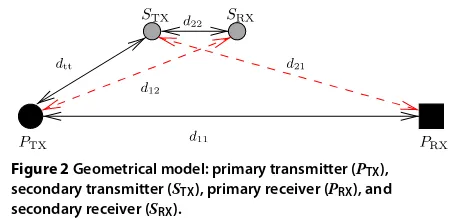
To present our results, we will use the simple geometrical model in Figure 2, in which the different nodes are placed on a plane. The relative positioning of the nodes is sum-marized by the distance between each pair of nodes. We model the block flat fading channel coefficient between two nodes as
Algorithm 3Algorithm to find the optimal parameters
1: forα←[ 0,. . ., 1]do 2: forP(11)←[ 0,. . .,P1
α]do
3: P(12)← P1−αP1(1) 1−α
4: K(11)←OPTIMAL-COVARIANCE(α,P(11)) 5: K(12)←P1(2)h11hH11
h112 6: forPr ←[ 0,. . .,P2]do
7: Kr←Prh21h
H
21 h212
8: ←
P(12)Pr h11h
H
21 h11h21
9: ObtainKp
10: ComputeR2
11: end for
12: end for
13: end for
vectors or matrices, each of the entries is independently modeled as in (38).
For convenience, we normalize all distances with respect to the distance between the primary users (i.e. d11 = 1). We will consider the square surface {(x,y) : x ∈[ 0, 1], y ∈[ 0, 1]}, and vary the position of the secondary nodes (relative to the primary nodes) over a regular square grid of size 11 × 11, that is, we will move the secondary transmitter and receiver over this grid, always parallel to the line between mary transmitter and receiver (as in Figure 2). The pri-mary transmitter and receiver will be fixed at positions (0, 0.5)(black filled circle) and(1, 0.5)(black filled box), respectively.
In the plots, a pair of coordinates (x,y) identifies the position of the secondary transmitter. All our results con-siderd22 = 1/4 while the remaining distances d12,d21 anddttvary as described before. This models a secondary middle-range communication in the presence of primary users.
5.2 Note on the strategies
The overlay strategy in Section 4.1 yields R2 = 0 for some channel realizations. The reason for this is that
Figure 2Geometrical model: primary transmitter (PTX), secondary transmitter (STX), primary receiver (PRX), and secondary receiver (SRX).
constraint (26b) cannot always be fulfilled forR2 > 0. In such a scenario, a cognitive radio system would switch to a different transmission strategy that can provide a non-zero secondary rateR2. For example, it could switch to the underlay transmission mode presented here. In this way, the hybrid overlay-underlay strategy would never perform worse than the pure underlay strategy. However, includ-ing such a functionality in our experiments is against the nature of our work, which is to compare the underlay and overlay scenarios, and evaluate the effect of the learning phase. For this reason, we implement the strategies exactly as described in Sections 3.1 and 4.1.
5.3 Complexity of the strategies
The complexity of the underlay solution varies for the different cases in Proposition 1, which depend on the instantaneous channel conditions. For cases 1 and 2, the complexity is that of solving one concave problem ((13) and (16), respectively). For case 3, the complexity is that of solving two concave problems: (16) (to check the constraint) and (18), and finding the optimal splitγ (e.g. using a loop or a bisection method). For MISO secon-daries, the complexity can be lowered (e.g. using Remark 2 and [14]).
In contrast, Algorithm 3 finds the optimal overlay trans-mission parameters by searching over three-real valued parameters defined on a closed and bounded space. Up to a scaling factor that depends on the powers, the matri-cesK(12),Kr and can be determined before hand. The covariance matrixK(11)needs to be determined for each pair(α, tr{K})using Algorithm 1. This algorithm relies on the waterfilling and bisection methods that can be imple-mented very efficiently (see e.g. [40]). In addition, note that Remark 5 can be used to minimize the number of calls to Algorithm 1. The optimalKpneeds to be determined for each triple(α,P(11),Pr)by solving the concave problem in (32), which can also be implemented efficiently. Solving this last problem can be avoided in the case whereKphas rank 1 using the results in Corollary 2.
When compared, it is clear that the complexity of solv-ing the overlay problem is significantly larger than that of the underlay problem, in particular for the case whereKp is not rank 1. Nevertheless, the solution to both problems reduces to solving concave problems, for which a large variety of efficient algorithms exist (see e.g. [38]).
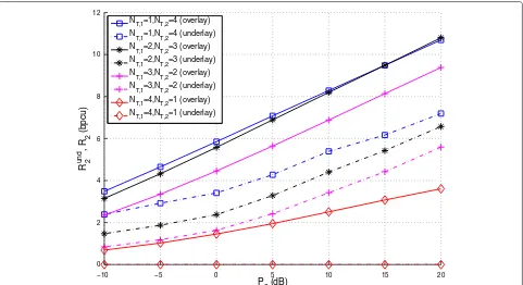
5.4 Simulation results
In the results in Figures 3, 4 and 5 the transmitters are equipped withNT,1 = NT,2 = 2 antennas, and the receivers with one single antenna. In contrast, in Figure 6, we study the behavior for varying NT,1 and NT,2 and single-antenna receivers. In all cases, the path loss expo-nent is fixed top=3, and the primary power is set toP1= 10 dB. The secondary power isP2=1 dB for the results in Figures 3 to 5 and variable for Figure 6. We assume that the primary system has a target rateR1 that corresponds to a fractionρ of its instantaneous point-to-point Shannon capacity, that is,
R1=ρlog(1+ h112P1). (39)
We refer toρ as the load factor of the primary system. We considerρ = 0.75 for Figures 3 to 5, andρ = 1 for Figure 6. Every point in the plots represents the average over 5·104independent realizations of the channels. We focus on the results for the overlay strategy and the com-parison between the strategies because the results for the underlay strategy alone do not differ qualitatively from the single-antenna case in [14].
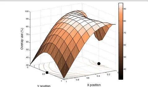
Figure 3 shows the average of the secondary rateR2(in bits per channel use, bpcu) achieved by our overlay cog-nitive radio strategy for NT,1 = NT,2 = 2,NR,2 = 1, P1 = 10 dB,P2 = 1 dB,p = 3 andρ = 0.75. To set the numerical values in the figure in a context note that if the secondaries were alone in the scenario, the ergodic
capacity would be 6.96 bpcu. In comparison, the high-est average secondary rate in Figure 3 isR2 = 6.29 bpcu and is obtained when primary and secondary transmitters are closely located. This represents 90% of the afore-mentioned capacity. As one would expect, the average secondary rate becomes lower as the two transmitters are separated.
It is more interesting to look at the advantage in average rate over the underlay strategy. Figure 4 shows the ratio between the average of the secondary rate for overlayR2 and the average of the secondary rate for underlayRund2 forNT,1 = NT,2 = 2,NR,2 = 1,P1 = 10 dB,P2 = 1 dB, p = 3 andρ = 0.75. The results are somewhat surpris-ing in the sense that the largest-advantage region does not correspond to the largest-secondary-rate region, that is, the maximum in Figure 4 is not obtained for(x,y) = (0, 0.5) but rather for(x,y) ≈ (0.4, 0.5). The reason for this is that for (x,y) = (0, 0.5), the underlay strategy also benefits from closely located transmitters, thanks to the interference decoding functionalities. In fact, if one removes this functionality in the underlay transmission mode, the results change significantly. In that case, the overlay system is overwhelmingly better than the underlay strategy.
In addition, note that the advantage of the overlay sys-tem diminishes as the two transmitters are separated. In fact, in some regions, using the underlay strategy is bet-ter in bet-terms of average secondary rate. The reason for
4
4
4
4.5
4.5
4.5
5
5
5
5.5
5.5
5.5
5.5 6
6
X position
Y position
0 0.1 0.2 0.3 0.4 0.5 0.6 0.7 0.8 0.9 1 0
0.1 0.2 0.3 0.4 0.5 0.6 0.7 0.8 0.9 1
0.8 0.9
0.9
1
1
1 1.1
1.1
1.1 1.2
1.2
1.2 1.2
1.2
1.3
1.3
1.3 1.3
1.3
1.4
1.4
1.4 1.4 1.4
X position
Y position
0 0.1 0.2 0.3 0.4 0.5 0.6 0.7 0.8 0.9 1 0
0.1 0.2 0.3 0.4 0.5 0.6 0.7 0.8 0.9 1
Figure 4Ratio of the average of the ratesR2(overlay) andRund2 (underlay).
0 0.2 0.4 0.6 0.8 1
0
0.5
1 30
40 50 60 70 80 90 100
X position Y position
Overlay use (%)
40 50 60 70 80 90
−10 −5 0 5 10 15 20 0
2 4 6 8 10 12
P2 (dB) R 2
und
, R
2
(bpcu)
N
T,1=1,NT,2=4 (overlay) N
T,1=1,NT,2=4 (underlay) N
T,1=2,NT,2=3 (overlay) N
T,1=2,NT,2=3 (underlay) N
T,1=3,NT,2=2 (overlay) N
T,1=3,NT,2=2 (underlay) N
T,1=4,NT,2=1 (overlay) N
T,1=4,NT,2=1 (underlay)
Figure 6Averaged ratesRund
2 (underlay) andR2(overlay) for different secondary powers and transmit antenna configurations.
this is simple: in these regions, the first phase is rela-tively long (e.g.α >0.5), and the higher sophistication of the secondary transmitter (i.e. dirty-paper coding, coop-erative transmission) cannot compensate for the loss in secondary rate due to the passive first phase. Thus, the underlay approach, even if it has to transmit mainly in the zero-forcing direction to avoid interference, can make a more efficient use of the resources and provide a larger rate to the secondary users.
In order to implement a system that combines both strategies (as discussed in Section 5.2), it is desirable to know how often they outperform each other. This is shown in Figure 5, in terms of the percentage of chan-nel realizations for which the overlay strategy yields a larger rate than the underlay strategy forNT,1 = NT,2 = 2,NR,2 =1,P1= 10 dB,P2 =1 dB,p=3 andρ =0.75. Again, we observe that the region with largest rate cor-responding to the overlay strategy does not correspond exactly to the collocation of transmitters. In the figure, we observe that, except for a small region where overlay is better over 90% of the time, there is room for significant improvement if the system implements both strategies and chooses the best one in each block.
Regarding variations in the scenario, we have observed the following general trends. The secondary rate (Figure 3) increases with both the number of antennas and the sec-ondary power as one would expect. More interestingly, as we increase the secondary power P2 or the number
of antennas, the maximum in Figure 4 (i.e. the advan-tage of overlay in terms of average rate) increases its value and shifts its position towards the primary transmitter. The load factor ρ is the parameter that has the most impact: the largest advantages of the overlay strategy are obtained for high primary load factors. For example, if ρ=1, the maximum advantage corresponds to a factor of approximately 2.55. In contrast, for small loads, the advan-tage might be too small to compensate for the additional complexity when compared to the underlay strategy; for example, in the case of a single-antenna primary system, we observed an advantage factor of just 1.15 (see [36]). Similar conclusions can be drawn for Figure 5: the max-imum tends to move towards the primary transmitter as we increase the secondary power or the number of anten-nas and the region where overlay is better most of the time becomes larger. Finally, for larger path losses (e.g. p=4), the results become more extreme: the positions of the maxima in Figures 3 to 5 remain the same, but their values are higher. In contrast, when the transmitters are separated, the underlay scheme yields a larger advantage than the one presented here.
p = 3. The secondary transmitter is placed at position (x,y) = (0.3, 0.5), i.e. on the line between the primary users. The main observation is that, in terms of secondary rate, it is better to deploy the antennas at the secondary transmitter rather than at the primary transmitter. In the underlay case, this is rather straightforward for the sec-ondary system cannot benefit from the antennas at the primary. In the overlay case, this observation implies that the gains obtained via spatial diversity (i.e. larger NT,2) increase faster than those obtained by shortening the learning phase (i.e. larger NT,1). However, observe that increasingNT,2suffers from a law of diminishing returns and that beyond a certain value the gains are minor. Regarding the changes in the behavior for varying sec-ondary powerP2, we observe the following general trends. For very lowP2, all the strategies are power-constrained, and thus the gap between underlay and overlay vanishes. This effect is more pronounced for ρ < 1, where the primary can tolerate some interference. The gap between the strategies widens asP2increases, meaning, than when the secondary transmitter is no longer power limited, the use of spatial shaping alone fails to exploit the available resources. A special, extreme case is the underlay strategy withNT,2 = 1: lacking spatial resources, it cannot make any use of a fully loaded primary channel, i.e. R2 = 0 independently ofP2.
6 Coexistence with MIMO primary systems The discussion in this paper has been restricted to the coexistence of a MIMO secondary system with a MISO primary link. The results presented here cannot be extended in their totality to the case of MIMO pri-maries neither for underlay nor for overlay. However, as we will see in this section, under some reasonable assump-tions, they carry over to scenarios with MIMO primary systems.
In the case of underlay cognitive radio, it is important to emphasize the underlying assumption that the pri-mary users are oblivious to the presence of secondary users. This effectively decouples the design of the optimal secondary transmitter from the primary transmit param-eters. Moreover, note that the effect of the primary users enters the optimization in (10) through constraints (10b) and (10c). The validity of Lemma 1 which plays a fun-damental role in dealing with the non-convexity of (10c) does not rely on any assumption about the primary trans-mit covariance matrix and thus applies to the primary MIMO case as well. In contrast, the simple transforma-tion of (10b) into a linear constraint (i.e. (40b)) is no longer possible in the MIMO primary case. If, however, this constraint is replaced by a constraint that is linear or convex in(K21,K21), then the results in Proposition 1 remain valid. For example, one may define a constraint analog to (10b) by considering the worst-interference
direction in the span of H21. Alternatively, if the pri-mary system uses single-stream transmission with fixed receiver beamformer, the results presented here remain valid.
In the case of the overlay cognitive radio strategy, the problem is more involved. In addition to a similar prob-lem regarding constraint (26c), the transmit strategies of primary and secondary systems are necessarily coupled by the very nature of the extended cognitive radio chan-nel (i.e. by the message-learning phase). Moreover, in the case of MIMO primaries, the optimization over the vir-tual joint covariance matrix Kco is more complex than in the case of MISO primaries, where beamforming was optimal, and thusKco could be determined easily. This is issue is especially important when considering efficient algorithms to find the optimal parameters. Notwithstand-ing these considerations, the results in this paper remain valid if the primary system uses single-stream transmis-sion with fixed receive beamformer, as in the case of underlay.
7 Conclusion
In this paper, we have studied the transmission strategies for underlay cognitive radio and overlay cognitive radio with an explicit learning phase, in which the secondary transmitter acquires the primary message. Our strategy for underlay uses interference decoding and exploits spa-tial resources using multi-antenna methods. For the over-lay case, we have combined cooperative communication techniques (decode-and-forward relaying) with commu-nication over a cognitive radio channel (cooperation and interference control at the primary receiver and interfer-ence pre-cancellation at the secondary transmitter) using multi-antenna methods. For both strategies, we have char-acterized the set of system parameters that maximize the secondary rate while ensuring a fixed rate for the primary system.
Appendices Appendix 1
Proof of proposition 1
We first prove an auxiliary lemma that will be used in the proof of Proposition 1. Note that using simple manipulations, the optimization problem in (10) can be reformulated as
max K2,1,K2,2
I+HH22(K2,1+K2,2)H22+HH12K1H12−Rund1,2 (40a)
subject to:
tr{hH21(K2,1+K2,2)h21} ≤Pundint , (40b)
Rund1,2 ≥R1, (40c)
tr{K2,1+K2,2} ≤P2, (40d)
K2,10,K2,20, (40e)
withPintundas defined in (14).
We will show now that when considering case 3, there is no loss of generality in restricting constraint (40c) to be an equality.
Lemma 1. Any optimal point that falls within case 3 can be attained by a pair of covariance matrices(K˜2,1,K˜2,2), such thatK˜2,2satisfies constraint(40c)with equality.
Proof. LetK2,1andK2,2solve the optimization problem and assume that
Rund1,2(K2,2) >R1, (41)
where the notation Rund1,2(K2,2) stresses out the dependency of Rund1,2 on K2,2. Similarly, the notation Rund2 (K2,1,K2,2)will stress out the dependency ofRund2 on
K2,1andK2,2.
First, we consider the case K2,1 = 0. Let be the solution to problem (16) (in case 2) and recall that
Rund1,2() <R1, (42)
Rund2 (0,K2,2)≤Rund2 (0,), (43)
for case 3. Now, construct the new covariance matrix ˜
K2,2=γK2,2+(1−γ ). (44)
Note that for anyγ ∈[ 0, 1], this matrix satisfies constrains (40b), (40d) and (40e), and
Rund2 (0,K2,2)≤Rund2 (0,K˜2,2), (45)
by the concavity property of the log-determinant. Rund1,2(K˜2,2)is a continuous function ofγ that satisfies
Rund1,2|γ=1=Rund1,2(K2,2) >R1>Rund1,2()=Rund1,2|γ=0. (46)
Thus, by choosingλappropriately, we construct either an admissible matrix that yields a higher secondary rate or
a matrix yielding the same secondary rate, and such that (40c) is satisfied with equality.
We now consider the case K2,1 = 0. Construct the following two covariance matrices
˜
K2,1=(1−γ )K2,1, (47)
˜
K2,2=K2,2+γK2,1 (48)
forγ ∈[ 0, 1]. Note that by construction, both K˜2,1and ˜
K2,2 are positive semi-definite. Moreover, this choice of covariance matrices satisfies
˜
K2,1+K˜2,2=K2,1+K2,2, (49)
and thus the constraints (40b), (40d) and (40e) are sat-isfied, and the first term in the objective function (40a) remains unchanged. However, noting that
|A+B+C| |B+C| ≤
|A+B|
|B| (50)
forA0,C0 andB0, we see that
Rund1,2(K2,2)≥Rund1,2(K˜2,2) (51)
for any γ ∈[ 0, 1]. Moreover, Rund1,2(K˜2,2) is a non-increasing and continuous function ofγ. If, for anyγ ∈ (0, 1], we have that
Rund1,2(K2,2) >Rund1,2(K˜2,2)≥R1, (52) then we have contradicted our initial hypothesis. Other-wise, by the non-increasing property, the pair of matrices
˜
K2,2=K2,2+K2,1andK˜2,1=0(i.e.γ =1) must also be a valid solution. Thus, we can use the first part of the proof to show that there is no loss of generality in restricting (40c) to be an equality.
We now proceed to prove Proposition 1.
Proof of Proposition 1. The proof for case 1 follows from the fact that it is not possible for the secondary receiver to decode the primary message (for the case of equality in (11), anyK2,2 =0would render decoding of the primary message impossible). Thus, the best that the transmitter can do is to choose the covariance matrix that maximizes (12). The formulation in (13) follows by noting that the denominator in (12) is independent from the covariance matrix.
To prove the solution for case 3, we make use of Lemma 1 to rewrite the optimization problem in (40) as
max
Note that only the first term in the objective function is relevant for the optimization. Moreover, except for (53c), the maximization only depends on K2,1,K2,2 through their sum, which we denote by . The general solution (K2,1,K2,2)can be obtained by computing the optimal disregarding constraint (53c) and then setting
K2,1=γ, (54)
K2,2=(1−γ ), (55)
with γ ∈[ 0, 1], such that Rund1,2 = R1. Note that suchγ must exist becauseRund1,2 is continuous inγ and
Rund1,2|γ=1<R1<Rund1,2|γ=0, (56) by assumption for case 3.
Appendix 2
Proof of proposition 2
We shall make use of the following well-known Lemma in our arguments:
appropriate dimensions) is strictly increasing inβ.
Proof.We have that
where λi and r are the singular values and the rank of
BHCB, respectively. It is easy to check that the first deriva-tive of each of the terms in the sum is posideriva-tive forβ >0, proving that (57) is strictly increasing inβ.
Proof of proposition 2. First, we prove statement 1 by contradiction. Assume that the set of parameters that attains the optimum satisfies
tr{Kp+Kr}<P2. (59)
Consider two new covariance matrices ˜ that do not violate constraint (26d) and such that R(12) evaluated forK˜pandK˜rremains unchanged (and hence satisfy (26c)). However, usingK˜pyields a larger secondary rateR2, which contradicts our assumption that the set of parameters solved the optimization problem.
We now prove statement 2 also by contradiction. Assume that the optimal choice of parameters yields
αtr{K(11)} +(1−α)tr{K(12)}<P1, (62) where K(11) is the optimal choice of covariance matrix. Now, define the matrixK˜(11) = γK(11) for someγ > 1, such that
αtr{K˜(11)} +(1−α)tr{K(12)} ≤P1. (63) This choice of matrix yields
˜
where λi and r are the singular values and the rank of
HtK(11)HHt, respectively. Thus, we have that ˜
R(11)+R(12)>R1 (74)
˜
Rt>R1, (75)
and we can find a shorter duration of the first phaseα < α˜ such that the rates, evaluated atα˜, satisfy
˜
R1(1)(α)˜ +R1(2)(α)˜ ≥R1, (76)
˜