R E S E A R C H
Open Access
Qualitative behavior of a rational difference
equation
yn+1=yn+yn−1 p+ynyn−1
Xiao Qian
*and Shi Qi-hong
* Correspondence:
This article is concerned with the following rational difference equationyn+1= (yn+ yn-1)/(p+ynyn-1) with the initial conditions;y-1, y0are arbitrary positive real numbers,
andp is positive constant. Locally asymptotical stability and global attractivity of the equilibrium point of the equation are investigated, and non-negative solution with prime period two cannot be found. Moreover, simulation is shown to support the results.
Keywords:Global stability attractivity, solution with prime period two, numerical simulation
Introduction
Difference equations are applied in the field of biology, engineer, physics, and so on [1]. The study of properties of rational difference equations has been an area of intense interest in the recent years [6,7]. There has been a lot of work deal with the qualitative behavior of rational difference equation. For example, Çinar [2] has got the solutions of the following difference equation:
xn+1=
axn−1
1 +bxnxn−1
Karatas et al. [3] gave that the solution of the difference equation:
xn+1=
xn−5
1 +xn−2xn−5
.
In this article, we consider the qualitative behavior of rational difference equation:
yn+1=
Let us introduce some basic definitions and some theorems that we need in what follows.
Lemma 1. LetIbe some interval of real numbers and f :I2→I
be a continuously differentiable function. Then, for every set of initial conditions,x-k,
x-k+1, ...,x0 ÎIthe difference equation
xn+1=f(xn,xn−1), n= 0, 1,. . . (2)
has a unique solution{xn}∞n=−k.
Definition 1 (Equilibrium point). A point x¯∈Iis called an equilibrium point of Equation 2, if
¯
x=f(x¯,x¯)
Definition 2 (Stability). (1) The equilibrium pointx¯ of Equation 2 is locally stable if for everyε> 0, there existsδ> 0, such that for any initial datax-k,x-k+1, ...,x0ÎI, with
|x−k− ¯x|+|x−k+1− ¯x|+· · ·+|x0− ¯x|< δ,
we have|xn− ¯x|< ε, for alln≥-k.
(2) The equilibrium point x¯ of Equation 2 is locally asymptotically stable if ¯x is locally stable solution of Equation 2, and there exists g> 0, such that for allx-k, x-k+1, ...,x0 ÎI, with
|x−k− ¯x|+|x−k+1− ¯x|+· · ·+|x0− ¯x|< γ,
we have
lim n→∞xn=x¯.
(3) The equilibrium point ¯xof Equation 2 is a global attractor if for allx-k,x-k+1, ...,
x0ÎI, we havenlim→∞xn=x¯..
(4) The equilibrium point ¯xof Equation 2 is globally asymptotically stable if ¯x is locally stable andx¯ is also a global attractor of Equation 2.
(5) The equilibrium point x¯of Equation 2 is unstable ifx¯ is not locally stable. Definition 3The linearized equation of (2) about the equilibrium x¯ is the linear dif-ference equation:
yn+1=
k
i=0
∂f(x¯,x¯,. . .,¯x)
∂xn−i yn−i (3)
Lemma 2[4]. Assume thatp1,p2ÎRandkÎ{1, 2, ...}, then
p1+p2<1,
is a sufficient condition for the asymptotic stability of the difference equation
xn+1−p1xn−p2xn−1= 0, n= 0, 1,. . . (4)
Moreover, suppose p2> 0, then, |p1| + |p2| < 1 is also a necessary condition for the asymptotic stability of Equation 4.
Lemma 3[5]. Let g:[p, q]2®[p, q] be a continuous function, wherepandqare real numbers withp<qand consider the following equation:
xn+1=g(xn,xn−1), n= 0, 1,. . . (5)
(1)g(x, y) is non-decreasing inxÎ[p, q] for each fixedyÎ [p, q], and g(x, y) is non-increasing in yÎ[p, q] for each fixedxÎ[p, q].
(2) If (m, M) is a solution of system
M =g(M, m) andm=g(m, M), then M=m.
Then, there exists exactly one equilibrium x¯ of Equation 5, and every solution of Equation 5 converges to x¯.
The main results and their proofs
In this section, we investigate the local stability character of the equilibrium point of Equation 1. Equation 1 has an equilibrium point
¯
Theorem 1. (1) Assume thatp> 2, then the equilibrium pointx¯= 0of Equation 1 is locally asymptotically stable.
(2) Assume that 0 <p< 2, then the equilibrium point x¯=2−pof Equation 1 is locally asymptotically stable, the equilibrium point x¯= 0is unstable.
Proof. (1) whenx¯= 0,
The linearized equation of (1) aboutx¯= 0is
yn+1−
1
pyn−
1
pyn−1= 0. (7)
It follows by Lemma 2, Equation 7 is asymptotically stable, ifp> 2. (2) when x¯=2−p,
It follows by Lemma 2, Equation 8 is asymptotically stable, if
p−21+p−1 2
Therefore,
0<p<2.
Equilibrium point x¯= 0is unstable, it follows from Lemma 2. This completes the proof.
Theorem 2. Assume thatv20<p<u20, the equilibrium pointx¯= 0andx¯=2−pof Equation 1 is a global attractor.
Proof. Let p, q be real numbers and assume that g:[p, q]2 ® [p, q] be a function defined by g(u,v)= u+v
p+uv, then we can easily see that the functiong(u, v) increasing inuand decreasing inv.
Suppose that (m, M) is a solution of system
M =g(M, m) andm=g(m, M). Then, from Equation 1
M= M+m
p+Mm, m=
M+m
p+Mm.
Therefore,
pM+M2m=M+m, (9)
pm+Mm2=M+m. (10)
Subtracting Equation 10 from Equation 9 gives
p+Mm(M−m)= 0.
Since p+Mm≠0, it follows that M=m.
Lemma 3 suggests that ¯xis a global attractor of Equation 1 and then, the proof is completed.
Theorem 3. (1) has no non-negative solution with prime period two for allpÎR+ . Proof. Assume for the sake of contradiction that there exist distinctive non-negative real numbersandψ, such that
. . .,ϕ,ψ,ϕ,ψ,. . .
is a prime period-two solution of (1). andψsatisfy the system
ϕp+ϕψ=ϕ+ψ, (11)
ψp+ϕψ=ψ+ϕ, (12)
Subtracting Equation 11 from Equation 12 gives
(ϕ−ψ)p+ϕψ= 0,
Numerical simulation
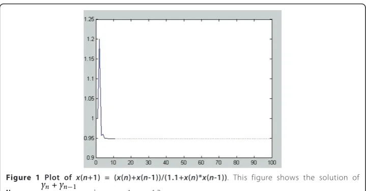
In this section, we give some numerical simulations to support our theoretical analysis. For example, we consider the equation:
yn+1=
yn+yn−1
1.1 +ynyn−1 (13)
yn+1=
yn+yn−1
1.5 +ynyn−1 (14)
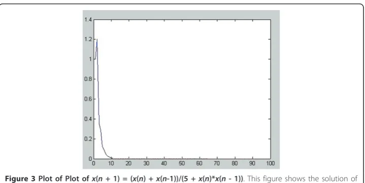
yn+1=
yn+yn−1
5 +ynyn−1 (15)
We can present the numerical solutions of Equations 13-15 which are shown, respec-tively in Figures 1, 2 and 3. Figure 1 shows the equilibrium point ¯x=√2−1.1of Equation 13 is locally asymptotically stable with initial data x0 = 1, x1 = 1.2. Figure 2 shows the equilibrium point x¯=√2−1.5 of Equation 14 is locally asymptotically Figure 1 Plot of x(n+1) = (x(n)+x(n-1))/(1.1+x(n)*x(n-1)). This figure shows the solution of
yn+1=
yn+yn−1
1.1 +ynyn−1
, wherex0= 1,x1= 1.2
Figure 2 Plot of x(n+1) = (x(n)+x(n-1))/(1.5+x(n)*x(n-1)). This figure shows the solution of
yn+1=
yn+yn−1
1.5 +ynyn−1
stable with initial datax0 = 1, x1 = 1.2. Figure 3 shows the equilibrium pointx¯= 0of Equation 15 is locally asymptotically stable with initial data x0= 1,x1= 1.2.
Authors’contributions
Xiao Qian carried out the theoretical proof and drafted the manuscript. Shi Qi-hong participated in the design and coordination. All authors read and approved the final manuscript.
Competing interests
The authors declare that they have no competing interests.
Received: 10 February 2011 Accepted: 3 June 2011 Published: 3 June 2011
References
1. Berezansky L, Braverman E, Liz E:Sufficient conditions for the global stability of nonautonomous higher order difference equations.J Diff Equ Appl2005,11(9):785-798.
2. Çinar C:On the positive solutions of the difference equationxn+1=axn-1/1+bxnxn-1.Appl Math Comput2004,
158(3):809-812.
3. Karatas R, Cinar C, Simsek D:On positive solutions of the difference equationxn+1=xn-5/1+xn-2xn-5.Int J Contemp
Math Sci2006,1(10):495-500.
4. Li W-T, Sun H-R:Global attractivity in a rational recursive sequence.Dyn Syst Appl2002,3(11):339-345. 5. Kulenovic MRS, Ladas G:Dynamics of Second Order Rational Difference Equations with Open Problems and
Conjectures.Chapman & Hall/CRC Press; 2001.
6. Elabbasy EM, El-Metwally H, Elsayed EM:On the difference equationxn+1=axn-bxn/(cxn-dxn-1).Adv Diff Equ2006,
1-10.
7. Memarbashi R:Sufficient conditions for the exponential stability of nonautonomous difference equations.Appl Math Lett2008,3(21):232-235.
doi:10.1186/1687-1847-2011-6
Cite this article as:Qian and Qi-hong:Qualitative behavior of a rational difference equation .Advances in Difference Equations20112011:6.
Figure 3Plot of Plot ofx(n+ 1) = (x(n) +x(n-1))/(5 +x(n)*x(n- 1)). This figure shows the solution of
yn+1=
yn+yn−1
5 +ynyn−1