A fractional order Legendre collocation method for solving the Bagley Torvik equations

(1)

R E S E A R C H

Open Access

A fractional-order Legendre collocation

method for solving the Bagley-Torvik

equations

Fakhrodin Mohammadi

1*

_{and Syed Tauseef Mohyud-Din}

2

*_{Correspondence:}

[email protected] 1_{Department of Mathematics,}

University of Hormozgan, P.O. Box 3995, Bandarabbas, Iran Full list of author information is available at the end of the article

Abstract

In this article, a numerical method based on the fractional-order shifted Legendre polynomials (FSLPs) and their operational matrix of fractional integration is

introduced for solving the fractional Bagley-Torvik equations. The main advantage of the presented method is that it can reduce a solution of the initial and boundary value problems for the fractional Bagley-Torvik differential equations to a system of algebraic equations. In order to confirm the efficiency and superiority of the presented method, some numerical examples are provided and a comparison is presented between the obtained results and those results achieved from other existing methods in the literature.

MSC: 26A33; 34A08; 65N35

Keywords: Bagley-Torvik equations; Riemann-Liouville fractional integration; fractional-order Legendre polynomials; operational matrix; collocation method

1 Introduction

Fractional calculus, the theory of differentiation and integration to non-integer order, is very useful for the description of various physical phenomena, such as damping laws, diffusion process, etc. Fractional derivatives provide an excellent instrument for the de-scription of memory and hereditary properties of various materials and processes [–]. Especially, fractional differential equations provide outstanding tools for illustration of many engineering and physical problems. Since most fractional differential equations do not have exact and analytic solutions, the accurate numerical techniques for solving these fractional equations are a challenging and motivational research area in mathematics and engineering.

The fractional Bagley-Torvik equation was originally formulated in a description of a real material by the use of fractional calculus. Moreover, the Bagley-Torvik equation has appeared in simulating the motion of a rigid plate immersed in a Newtonian ﬂuid [–]. This equation has been studied both analytically and numerically in []. Diethelm [] transformed this equation into a system of fractional diﬀerential equation and solved the problem with the Adams predictor and the corrector method. Recently, considerable at-tention has been devoted to numerical solutions of the fractional Bagley-Torvik equation. For example the spectral tau method [, ], the operational formulation of collocation

(2)

methods [, ], collocation methods [–], wavelet methods [, ], pseudospectral methods [], diﬀerential transform methods [], hybrid functions methods [], and fractional Taylor methods [] have been used to solve this fractional diﬀerential equa-tion. In this study, a fractional-order Legendre collocation method is proposed for solving the Bagley-Torvik equations.

Applications of orthogonal functions and polynomials for numerical solution of ordi-nary differential equations refer, at least, to the time of Lanczos []. Moreover, the origin of some current spectral method, such as the Galerkin, tau, and pseudospectral methods can be found in the ‘weighted residual method’ of Finlayson and Scriven []. Nowadays, spectral methods are efficient techniques for solving a different kind of fractional differ-ential and integral equations accurately [, , , ]. The main advantage of spectral methods lies in their accuracy for a given number of unknowns. For smooth problems in simple geometries, they offer exponential rates of convergence (spectral accuracy). By us-ing the operational matrices for basis functions, spectral methods reduce the solution of fractional differential and integral equations into a solution of systems of algebraic equa-tions which produce highly accurate soluequa-tions for these equaequa-tions [, , , ].

This paper is structured as follows: In Section  some basic preliminaries of the frac-tional calculus are presented. The FSLPs and their properties are introduced in Section . Section  is devoted to an operational matrix of fractional integration for the FSLPs. Ap-plication of the FSLPs for solving the Bagley-Torvik equation is considered in Section . Convergence and an error estimate for the FSLPs expansion are given in Section . The eﬃciency and superiority of the proposed method is demonstrated by considering some numerical examples in Section . Finally, a conclusion is given in Section .

2 Preliminaries

In this section we review some basic deﬁnitions and preliminaries of the fractional calculus which are used in the next sections.

2.1 Fractional calculus

Fractional-order calculus is a branch of calculus which deals with integration and diﬀeren-tiation operators of non-integer order. Among the several formulations of the generalized derivative, the Riemann-Liouville and Caputo deﬁnition are most commonly used, which can be described as follows [].

Deﬁnition  A real functionf(t),t> , is said to be in the spaceCμ,μ∈Rif there exist

a real numberp>μand a functionf(t)∈C[,∞) such thatf(t) =tpf(t), and it is said to

be in the spaceCn

μ,n∈Niff(n)∈Cμ.

Deﬁnition  The Riemann-Liouville fractional integration of orderν≥ of a function

f ∈Cμ,μ≥–, is deﬁned as

Jν

f(t) =



(ν)

t

(t–τ)

ν–_f₍_τ₎_d_τ_, _ν_{> ,}

f(t), ν= .

The Riemann-Liouville fractional operatorJν_{has the following properties:}

JνJν_f₍_t₎₌JνJν_f₍_t₎_, _ν

(3)

JνJν_f₍_t₎₌Jν+ν_f₍_t_), _ν

,ν≥,

Jν_tλ₌ (λ+ ) (λ+ν+ )t

ν+λ_, _ν_≥_,_λ_{> –.}

Deﬁnition  The fractional derivative of orderν>  in the Caputo sense is deﬁned as

Dν

erties of the Caputo fractional operatorsDν_{are given by the following expressions:}

Jν

For more details of fractional calculus and their applications please refer to [–].

3 The FSLPs and their properties

The FSLPs can be deﬁned based on the deﬁnition of the shifted Legendre polynomials by introducing the change of variablet=xα_for_α_{>  []. Let}_P

n(x) is thenth shifted Leg-endre polynomial andP(n,α)(x) denote thenth FSLPs,i.e. Pn(xα). By using the recurrence formula for the shifted Legendre polynomials, it can be given as

(4)

Any functionf(t) deﬁned over [, ] may be expanded in terms of FSLPs as

in which theckare derived by

ck=α(k+ )





P(m,α)(x)P(n,α)(x)wα(x)dx.

If the inﬁnite series in equation () is truncated, then it can be written as

f(x)fM(x) =

4 Operational matrix of fractional integration of FSLPs

In recent years various operational matrices for the polynomials have been developed to cover the numerical solution of differential, integral and integro-differential equations. The main advantage of these operational matrices is that they replace differential and in-tegral operators with some matrices. Consequently, they reduce such problems to those of solving a system of algebraic equations, greatly simplifying the problem [–]. In this section the operational matrix of fractional integration for FSLPs will be derived.

Theorem . The Riemann-Liouville fractional integration of orderνfor the M×FSLPs vectorα(x)can be deﬁned as

Now the termxαr_{is expanded exactly by FSLPs as}

xαr= M–

j=

(5)

in which theρr,scan be derived as

By substituting equations () and () in () we have

Jν

this means that the fractional integration ofith element ofα(x) can be expanded in FSLPs

as derived in equation () and this yields the desired result directly.

5 Numerical solution of Bagley-Torvik equations The fractional Bagley-Torvik equation is of the form

ADy(x) +ADνy(x) +Ay(x) =f(x), ≤x≤R,  <ν< , ()

subject to the initial conditions

y() =α, y() =α, ()

or the boundary conditions

y() =β, y(R) =β, ()

whereA,A,A,α,α,β, andβare constants withA= . To solve this fractional

Bagley-Torvik equation we consider two cases.

Case () Intitial conditions: For solving the Bagley-Torvik equation () with intitial con-ditions (), we use the change of variablet=x_Rto transformx∈[,R] int∈[, ]. So, we

subject to the initial conditions

Y() =α, Y() =Rα, ()

in whichY(t) =y(Rt) andF(t) =f(Rt). Now, we approximate the functionsY(t) andF(t) in terms of FSLPs as

(6)

where Cis an unknownM× vector. Substituting equation () in equation () and applying the Riemann-Liouville integral operatorJ_{we get}

A

by using the operational matrix of fractional integrationM(ν)_{we have}

A

Now we collocate the equation () at theMzeros of the shifted Legendre polynomial

PM(x). This generates a system ofMalgebraic equations for the unknown vectorC. After ﬁnding the solution of this algebraic system, the solutionY(t) can be derived by substitut-ing the vectorCin equation ().

Case () Boundary conditions: To solve the Bagley-Torvik equation () with boundary conditions (), similar to the previous case, by using the change of variablet=x_Rwe obtain

A

substituting the approximation functionsY(t) andF(t) deﬁned in equation () into equa-tion () and using the operaequa-tional matrix of fracequa-tional integraequa-tionM(ν)_{we get}

A at theMzeros of the shifted Legendre polynomialPM(x) and this gives a system ofM algebraic equations for the unknown vectorC. Moreover, the boundary conditiony(R) =

Y() =βgive a linear equation. This equation together withMalgebraic equations derived

(7)

6 Error analysis

In this section, in order to demonstrate the eﬃciency of the proposed FSLPs method, we have given some theorems on convergence and error estimation. The next theorem gives an upper bound for the error function of the truncated FSLPs series.

Theorem . Let f(x)be a deﬁned function on[, ] and g(x) =f(xα)∈Cn+[, ],the

mean error bound for the truncated FSLPs series fM(x) =

M–

M–  which approximatesf(x) with minimum mean error, so

f–fM α=

in which Qn(x) is the well-known polynomial interpolation for g(t) at shifted zeros of Chebyshev polynomials in the interval [, ]. Now by using an error bound of the poly-nomial interpolationQn(t) (Theorem . in []) we have

taking the square root of both sides completes the proof.

Now, we give the error estimation of the numerical method given in the previous section. Supposey(x) is the exact solution of () andyM(x) is the approximate solution fory(x). Here, we introduce a process for estimating the error of the approximate solution,i.e. eM(x) =y(x) –yM(x). Consider the perturbation functionRM(x), depending only on the approximate solutionyM(x) as

RM(x) =ADy(x) +ADνy(x) +Ay(x) –f(x), ()

subtracting () from () we obtain

ADeM(x) +ADνeM(x) +AeM(x) =RM(x), ()

these Bagley-Torvik equations with initial conditionseM() = ,eM() =  or boundary conditions eM() = ,eM(R) =  can be solved by using the proposed FSLPs method as given in previous section for this system to ﬁnd an approximation of the error function

(8)

7 Numerical examples

In this section, the eﬃciency and superiority of the proposed method is demonstrated by some illustrative examples. All algorithms are performed by Maple .

Example  Let us consider the Bagley-Torvik equation () with the following conditions [, , ]:

A=A=A= , ν= ., ≤x< , f(x) =x+ ,

y() = , y() = .

The exact solution of this problem is

y(x) =x+ .

The FSLPs basis and its fractional operational matrix have been applied for solving this fractional Bagley-Torvik equation. Forα=  andM=  the presented FSLPs collocation method results in the following linear system for the unknownsc,c, andw:

⎧ ⎪ ⎪ ⎪ ⎪ ⎪ ⎪ ⎨ ⎪ ⎪ ⎪ ⎪ ⎪ ⎪ ⎩

.w– .c+ .c

– . = ,

–.w– .c+ .c

– . = ,

c+c–  = ,

in whichw=y() andy(x) =cP(,α)(x) +cP(,α)(x). Solving this linear system we obtain

c= ., c= .,

w= ..

Hence, we gety(x) =  +xup to  digits precision which is the exact solution.

Example  In this example, we consider the Bagley-Torvik equation () with the follow-ing conditions [, , ]:

A= , A=A= , ν= ., ≤x< ,

f(x) =

√

x

√ π +t

_–_t_, _y_{() =}_y_{() = .}

y(x) =x–x.

(9)

following linear system:

Example  In this example, we consider the Bagley-Torvik equation () with the follow-ing conditions [, , ]:

y(x) =x–x

Similar to the previous examples the FSLPs method has been used for solving this problem. After solving the linear system derived by the presented collocation method forα=  and

M=  we get the following values for the unknown coeﬃcients:

c= ., c= –.,

c= ., c= .,

c= –., c= .,

(10)

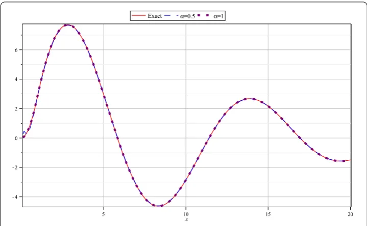
Figure 1 The exact and approximate solution forα= 0.5, 1 andM= 20.

and this results in

y(x) = .x– .x+ .x

– .x+ .x+ .×–, which is the exact solution up to  digits precision.

Example  In this example, we consider the Bagley-Torvik equation () with the follow-ing conditions []:

A= , A=A= , ν= ., ≤x< ,

f(x) =

√

x

√ π +x

₊_x_, _y_{() = ,} _y_{() = .}

y(x) =x.

Similar to the previous examples the FSLPs method has been used for solving this problem and by solving the linear system derived by the presented collocation method forα=  and

M=  we get

c= ., c= .,

c= ., c= –.×–.

and this results in the solution function in the interval [, ] as

(11)

(a)

(b)

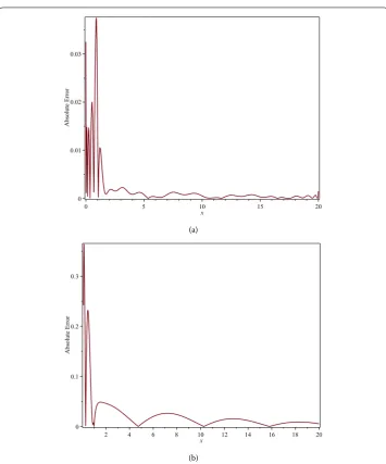
Figure 2 The absolute error of the obtained results.We took(a)α= 1 and(b)α= 0.5.

By the change of variablet=x_in this function we get

.x– .–x+ .×–,

which is the exact solution up to  digits precision.

Example  Consider the fractional Bagley-Torvik equation () with the following con-ditions [, –]:

A= , A= ., A= ., ν= ., ≤x< ,

y() = , y() = , f(x) =

(12)

Table 1 Comparison of the numerical solution forν= 1.5,α= 0.5, 1, andM= 17 with other results in [23, 27]

t Exact FSLPs (α= 0.5) FSLPs (α= 1.0) Ref. [27] Ref. [23]

1.40625 4.85696 4.80915 4.85715 4.95531 4.67105

2.03125 6.83165 6.78579 6.85062 6.93440 6.48436

2.96875 7.67925 7.64470 7.67261 7.80605 7.21918

3.59375 6.97278 6.94967 6.98356 7.09830 6.51938

4.21875 5.48313 5.47278 5.48883 5.59310 5.09093

5.46875 1.28657 1.29947 1.28343 1.33675 1.11881

7.96875 –4.53369 –4.50974 –4.53926 –4.59731 –4.30082

9.53125 –3.64404 –3.63542 –3.64279 –3.71142 –3.40603

11.7188 0.59143 0.57883 0.59421 0.58569 0.61398

13.5938 2.64127 2.62760 2.63996 2.67926 2.51628

15.4688 1.72175 1.71945 1.72207 1.75636 1.60585

16.4063 0.63025 0.63383 0.62882 0.64944 0.56273

17.3438 –0.44428 –0.43668 –0.44270 –0.44298 –0.45529

18.9063 –1.50186 –1.49344 –1.49966 –1.52298 –1.44138

19.8438 –1.52304 –1.51713 –1.518921 –1.54859 –1.44734

The exact solution of equation is given by

y(x) =

The proposed FSLPs collocation method is implemented for solving this fractional Bagley-Torvik equation. Figure  shows the exact and approximate solution forα= .,  andM= . The absolute errors for the obtained numerical solutions withα= . andα=  are plotted in Figure . Moreover, a comparison between the results achieved by the proposed FSLPs method withM=  and other methods in Refs. [, ] is presented in Table . From Table  we can immediately see that the FSLPs method, in comparison to other existing methods, is more eﬃcient and accurate.

8 Discussion and conclusion

A new type of orthonormal fractional-order Legendre polynomials is deﬁned. The oper-ational matrix of fractional integration for this fractional-order basis is derived. By using this fractional operational matrix and collocation method a numerical method is proposed for solving the fractional Bagley-Torvik equations. A comparison is made between nu-merical results derived by the presented collocation method and other existing nunu-merical method. According to the numerical results, we can conclude that the presented method is more accurate and eﬀective for a numerical solution of the fractional Bagley-Torvik equations.

Competing interests

(13)

Authors’ contributions

All authors participated in drafting, revising, and commenting on the manuscript. Also, all authors read and approved the ﬁnal draft of the manuscript.

Author details

1_{Department of Mathematics, University of Hormozgan, P.O. Box 3995, Bandarabbas, Iran.}2_{Department of Mathematics,}

HITEC University, Taxila Cantt, Pakistan.

Acknowledgements

We express our sincere thanks to the anonymous referees for valuable suggestions that improved the ﬁnal manuscript.

Received: 5 September 2016 Accepted: 7 October 2016 References

1. Kilbas, AA, Srivastava, HM, Trujillo, JJ: Theory and Applications of Fractional Diﬀerential Equations. Elsevier, San Diego (2006)

2. Oldham, KB, Spanier, J: The Fractional Calculus. Academic Press, New York (1974) 3. Podlubny, I: Fractional Diﬀerential Equations. Academic Press, San Diego (1999)

4. Golmankhaneh, AK, Golmankhaneh, AK, Baleanu, D: On nonlinear fractional Klein-Gordon equation. Signal Process.

91(3), 446-451 (2011)

5. Baleanu, D, Golmankhaneh, AK, Golmankhaneh, AK: Solving of the fractional non-linear and linear Schrödinger equations by homotopy perturbation method. Rom. J. Phys.54(10), 823-832 (2009)

6. Bhrawy, AH, Zaky, MA, Baleanu, D: New numerical approximations for space-time fractional Burgers’ equations via a Legendre spectral-collocation method. Rom. Rep. Phys.67, 340-349 (2015)

7. Bhrawy, AH, Baleanu, D: A spectral Legendre-Gauss-Lobatto collocation method for a space-fractional advection diﬀusion equations with variable coeﬃcients. Rep. Math. Phys.72, 219-233 (2013)

8. Bhrawy, AH: A new spectral algorithm for a time-space fractional partial differential equations with subdiffusion and super diffusion. Proc. Rom. Acad., Ser. A : Math. Phys. Tech. Sci. Inf. Sci.17, 39-46 (2016)

9. Bhrawy, AH: A Jacobi spectral collocation method for solving multi-dimensional nonlinear fractional sub-diﬀusion equations. Numer. Algorithms73, 91-113 (2016)

10. Kazem, S, Abbasbandy, S, Kumar, S: Fractional-order Legendre functions for solving fractional-order diﬀerential equations. Appl. Math. Model.37(7), 5498-5510 (2013)

11. Torvik, PJ, Bagley, RL: On the appearance of the fractional derivative in the behavior of real materials. J. Appl. Mech.

51, 294-298 (1984)

12. Bagley, RL, Torvik, PJ: A theoretical basis for the application of fractional calculus to viscoelasticity. J. Rheol.27(3), 201-210 (1983)

13. Yan, T, Luo, S: Local polynomial smoother for solving Bagley-Torvik fractional diﬀerential equations.Preprints

2016080231 (2016). doi:10.20944/preprints201608.0231.v1

14. Diethelm, K, Ford, J: Numerical solution of the Bagley-Torvik equation. BIT Numer. Math.42(3), 490-507 (2002) 15. Baleanu, D, Bhrawy, AH, Taha, TM: Two eﬃcient generalized Laguerre spectral algorithms for fractional initial value

problems. Abstr. Appl. Anal.2013, Article ID 546502 (2013)

16. Bhrawy, AH, Hafez, RM, Alzahrani, EO, Baleanu, D, Alzahrani, AA: Generalized Laguerre-Gauss-Radau scheme for the ﬁrst order hyperbolic equations in a semi-inﬁnite domain. Rom. J. Phys.60, 918-934 (2015)

17. Bhrawy, AH, Taha, TM, Alzahrani, EO, Baleanu, D, Alzahrani, AA: New operational matrices for solving fractional diﬀerential equations on the half-line. PLoS ONE10(9), e0138280 (2015). doi:10.1371/journal.pone.0126620 18. Bhrawy, AH, Abdelkawy, MA, Alzahrani, AA, Baleanu, D, Alzahrani, EO: A Chebyshev-Laguerre Gauss-Radau

collocation scheme for solving time fractional sub-diﬀusion equation on a semi-inﬁnite domain. Proc. Rom. Acad., Ser. A : Math. Phys. Tech. Sci. Inf. Sci.16, 490-498 (2015)

19. Cenesiz, Y, Keskin, Y, Kurnaz, A: The solution of the Bagley-Torvik equation with the generalized Taylor collocation method. J. Franklin Inst.347(2), 452-466 (2010)

20. Yuzbasi, S: Numerical solution of the Bagley-Torvik equation by the Bessel collocation method. Math. Methods Appl. Sci.36(3), 300-312 (2013)

21. El-Gamel, M, El-Hady, AM: Numerical solution of the Bagley-Torvik equation by Legendre-collocation method. SeMA J. (2016). doi:10.1007/s40324-016-0089-6

22. Mohammadi, F: Numerical solution of Bagley-Torvik equation using Chebyshev wavelet operational matrix of fractional derivative. Int. J. Adv. Appl. Math. Mech.2(1), 83-91 (2014)

23. Ray, SS: On Haar wavelet operational matrix of general order and its application for the numerical solution of fractional Bagley-Torvik equation. Appl. Math. Comput.218(9), 5239-5248 (2012)

24. Esmaeili, S, Shamsi, M: A pseudo-spectral scheme for the approximate solution of a family of fractional diﬀerential equations. Commun. Nonlinear Sci. Numer. Simul.16, 3646-3654 (2011)

25. Arikoglu, A, Ozkol, AI: Solution of fractional diﬀerential equations by using diﬀerential transform method. Chaos Solitons Fractals34, 1473-1481 (2007)

26. Mashayekhi, S, Razzaghi, M: Numerical solution of the fractional Bagley-Torvik equation by using hybrid functions approximation. Math. Methods Appl. Sci.39(3), 353-365 (2016)

27. Krishnasamy, VS, Razzaghi, M: The numerical solution of the Bagley-Torvik equation with fractional Taylor method. J. Comput. Nonlinear Dyn.11(5), 051010 (2016)

28. Lanczos, C: Trigonometric interpolation of empirical and analytical functions. J. Math. Phys.17, 123-129 (1938) 29. Finlayson, A, Scriven, LE: The method of weighted residuals: a review. Appl. Mech. Rev.19, 735-748 (1966) 30. Doha, EH, Bhrawy, AH, Ezz-Eldien, SS: A Chebyshev spectral method based on operational matrix for initial and

boundary value problems of fractional order. Comput. Math. Appl.62(5), 2364-2373 (2011)

(14)

32. Ezz-Eldien, SS, Hafez, RM, Bhrawy, AH, Baleanu, D, El-Kalaawy, AA: New numerical approach for fractional variational problems using shifted Legendre orthonormal polynomials. J. Optim. Theory Appl. (2016).

doi:10.1007/s10957-016-0886-1

33. Saadatmandi, A: Bernstein operational matrix of fractional derivatives and its applications. Appl. Math. Model.38, 1365-1372 (2014)

34. Saadatmandi, A, Dehghan, M: A new operational matrix for solving fractional-order diﬀerential equations. Comput. Math. Appl.59(3), 1326-1336 (2010)

35. Bhrawy, AH, Aloﬁ, AS: The operational matrix of fractional integration for shifted Chebyshev polynomials. Appl. Math. Lett.26, 25-31 (2013)

36. Doha, EH, Bhrawy, AH, Ezz-Eldien, SS: A new Jacobi operational matrix: an application for solving fractional diﬀerential equations. Appl. Math. Model.36, 4931-4943 (2012)

37. Doha, EH, Bhrawy, AH, Ezz-Eldien, SS: A Chebyshev spectral method based on operational matrix for initial and boundary value problems of fractional order. Comput. Math. Appl.62, 2364-2373 (2011)

38. Bhrawy, AH, Zaky, MA: Shifted fractional-order Jacobi orthogonal functions: application to a system of fractional diﬀerential equations. Appl. Math. Model.40, 832-845 (2016)