R E S E A R C H
Open Access
Initial value problem for second-order
random fuzzy differential equations
Ho Vu
1*and Le Si Dong
2*Correspondence: [email protected] 1Division of Computational
Mathematics and Engineering, Institute for Computational Science, Ton Duc Thang University, Ho Chi Minh City, Vietnam
Full list of author information is available at the end of the article
Abstract
In this paper the second-order random fuzzy differential equations (SRFDEs) under generalized Hukuhara differentiability are introduced. Under suitable conditions we obtain the existence and uniqueness results of solutions to an SRFDE. To prove this assertion we use the idea of successive approximations. Some examples are given to illustrate these results.
Keywords: fuzzy random variables; random fuzzy differential equations;
second-order random fuzzy differential equations; generalized Hukuhara derivative
1 Introduction
The study of fuzzy differential equations (FDEs) forms a suitable setting for the mathemat-ical modeling of real-world problems in which uncertainties or vagueness pervade. Most practical problems can be modeled as FDEs [, ]. Therefore, FDEs are a very important topic both in theory and application, for example, in population models, in engineering, in chaotic systems and in modeling hydraulics. Differentiability of fuzzy-valued functions was first introduced by Chang and Zadeh [], and followed by Dubois and Prade [], who defined and used the extension principle []. Other approaches have been discussed by Puri and Ralescu [], which generalized and extended the concept of Hukuhara differen-tiability for set-valued mappings to the class of fuzzy mappings. In this setting the fuzzy differential equations can be viewed as an abstract differential equation via embedding the fuzzy number space into Banach space. In this framework, many papers concerned with the existence and uniqueness problems. The problem of the existence and uniqueness be-gins with the investigations of Kaleva (see []) for the fuzzy Volterra integral equation that is equivalent to the initial value problem for fuzzy differential equations, where the Lipschitz condition and the Banach fixed point theorem and the method of successive approximations are applied in the problem of the existence and uniqueness of the solu-tion. Wuet al.[, ] and Song and Wu [] changed the initial value problem of fuzzy differential equations into abstract differential equations on a closed convex cone in a Ba-nach space by the operatorj, that is, the isometric embedding from (Ed,D) onto its range
in the Banach spaceX. They established the relationship between a solution and its ap-proximate type and dissipative-type conditions. Lupulescu [] established a new concept of inner product on the fuzzy space. By help of these concepts author formulated some dissipative conditions for fuzzy initial value problem and, under these conditions, author
established the global existence and uniqueness of a solution of fuzzy differential equa-tions. In the last few years, many researchers have worked on the theoretical of fuzzy dif-ferential equations [–] and other recent works such as the study of some topological properties and structure of the solutions to the Cauchy problem for fuzzy differential sys-tems (see [, ]). Subsequently, some very important extensions of the fuzzy differential equations based on H-derivative are the fuzzy functional differential equations [], the random fuzzy differential equations [], the fuzzy neutral differential equations [], and the fuzzy fractional differential equations [, ]. However, the approach using Hukuhara differentiation suffers a grave disadvantage,i.e., the solution has the property that the di-ameterdiam[x(t)]αis nondecreasing int, and so it is very hard to get any deep results on qualitative theory for fuzzy differential equations, such as asymptotic property, periodic-ity, bifurcation. Furthermore, Bede [] proved that a large class of two-point boundary value problems have no solutions at all under H-differentiability.
Recently, Bedeet al.[–] and Stefanini and Bede [] solved the above mentioned approach under strongly generalized differentiability of fuzzy-number-valued functions and studied fuzzy initial valued for the fuzzy differential equations involving strongly gen-eralized differentiability. In this case the derivative exists and the solutions of fuzzy differ-ential equations may have decreasing diameters, but the uniqueness is lost. Thus, almost all important discussions on the qualitative problems for FDEs are deduced in the frame-work of this approach (see [, , ]). Therefore, our point is that the generalization of the concept of H-differentiability can be of great help in the dynamic study of fuzzy differ-ential equations and random fuzzy problems. In [], first-order linear fuzzy differdiffer-ential equation under generalized differentiability concept are considered and solutions of this problem in some especial cases were presented. See also [, ] Malinowski studied two kinds of solutions to random fuzzy initial value problem under strongly generalized differ-entiability. In [] a linear fuzzy nuclear decay equation under generalized differentiability is studied and numerical solutions are found. Meanwhile, Allahviranlooet al.[–] and Khastanet al.[] have solved these FDEs in the sense of generalized derivatives. Subse-quently, some extensions of the fuzzy differential equations based on generalized differen-tiability are the fuzzy functional integro-differential equations [] and the random fuzzy integro-differential equations [–].
Random fuzzy differential equations (RFDEs) deal with the real phenomena, not only with randomness but also with fuzziness. Puri and Ralescu introduced a fuzzy-set-valued random variable in [], and gave the concept of differentiability by Hukuhara difference in []. In the literature, one can find various definitions of fuzzy random variables. For the first time the concept of a fuzzy random variable was proposed by Kwakernaak []. Further, it was used by Kruse and Meyer []. In [, ], there appear two notions of measurability of fuzzy mappings. The relations between different concepts of measurabil-ity for fuzzy random variables are contained in the papers of Colubiet al.[], Terán Agraz [], López-Díaz and Ralescu []. In this paper, we will use a definition of fuzzy random variable which was introduced by Puri and Ralescu []. This definition is currently the one most often used in probabilistic and statistical aspects of the theory of fuzzy random variables.
In [, ], the authors considered the random fuzzy differential equation with initial value
x(t,ω)[t,t=+p],P.fω
wheref:×[t,t+p]×Ed→Edand the symboldenotes the fuzzy derivative is
under-stood in the sense of Puri and Ralescu []. Malinowski also showed that iff is continuous andfω(t,x) satisfies the Lipschitz condition with respect tox, then there exists a unique local solution for the random fuzzy initial value problem (.). In [] the existence and uniqueness of the solution for RFDEs with non-Lipschitz coefficients is proven. Further-more, using generalized Hukuhara differentiability, Malinowski [, ] studied two kinds of solutions to (.) under condition that the right-hand side of equation is Lipschitzian and generalized Lipschitz. Author established the local and global existence and unique-ness results for (.) by using the method of successive approximations. Besides, in fact, a large class of physically important problem is described by fuzzy random differential systems. We believed that mathematical models of physical phenomena should have the properties that existence and uniqueness of solution and the solution’s behavior changes continuously with the initial conditions. The importance of existence and uniqueness the-orems in the study of initial value problems is well known due to their relevance in estab-lishing the well-posedness of the real-world problems arising in physical and engineering systems. Uniqueness results play a significant role in the continuation of solutions and in the theory of autonomous systems. While the uniqueness results almost always come at the cost of stringent conditions, they are valuable, for without such uniqueness results it is impossible to make predictions about the behavior of physical systems. Therefore, in this paper, we consider the second-order random fuzzy differential equation initial value problem of the form
D,Hgx(t,ω)[t,t=+p],P.fω(t,x(t,ω),D,Hgx(t,ω)),
x(t,ω)P=.I(ω), D,Hgx(t,ω)P=.I(ω)∈Ed,
(.)
wheref :×[t,t+p]×Ed×Ed→Edand the symbolD,Hg denotes the second-order
generalized Hukuhara derivative. The purpose of this article is to discuss the behaviors of solutions to the second-order random fuzzy differential equations under generalized Hukuhara differentiability, such as the existence and uniqueness of solutions, and that the solution’s behavior changes continuously with the initial conditions, which are important in the theory of fuzzy stochastic dynamical system analysis.
In this paper, we study four kinds of solutions to SRFDEs. The different types of solutions to SRFDEs are generated by the usage of two different concepts of the fuzzy derivative. We were inspired and motivated by the results of Bede and Gal [], Malinowski [, , ], and Allahviranlooet al.[] concerning deterministic FDEs with generalized fuzzy derivative and recently by the paper of Stefanini and Bede [] where two types of solutions to interval differential equations were investigated.
2 Preliminaries
In this section, we give some notations and properties related to fuzzy set space, and sum-marize the major results for integration and differentiation of fuzzy-set-valued mappings. We recall also the notations of fuzzy random variable and fuzzy stochastic process. Let
Kc(Rd) denote the family of all nonempty, compact and convex subsets ofRd. The
addi-tion and scalar multiplicaaddi-tion inKc(Rd) are defined as usual,i.e., forA,B∈Kc(Rd) and λ∈R,
A+B={a+b|a∈A,b∈B}, λA={λa|a∈A}.
The Hausdorff distance or Pompeiu-Hausdorff distancedHinKc(Rd) is defined as follows:
dH(A,B) =max
sup
a∈A
inf
b∈Ba–b,supb∈Bainf∈Aa–b
,
whereA,B∈Kc(Rd), and · denotes usual Euclidean norm inRd. It is well known (see
[]) thatKc(Rd) is a complete, separable, and locally compact metric space with respect
todH. DefineEd={u:Rd→[, ] such thatu(z) satisfies (i)-(iv) stated below}:
(i) uis normal, that is, there existsz∈Rdsuch thatu(z) = ;
(ii) uis fuzzy convex,i.e.,u(λz+ ( –λ)z)≥min{u(z),u(z)}for anyz,z∈Rdand λ∈[, ];
(iii) uis upper semicontinuous;
(iv) [u]=cl{z∈Rd:u(z) > }is compact, wherecldenotes the closure in(Rd, · ).
Elements ofEd are often called fuzzy sets ofRd. Forα∈(, ], define [u]α={z∈Rd| u(z)≥α}. We will call this set an α-cut (α-level set) of the fuzzy set u. For u∈ Ed
one has [u]α ∈K
c(Rd) for every α ∈[, ]. For two fuzzy sets u,u∈Ed, we denote u≤u if and only if [u]α⊂[u]α. Ifg:Rd×Rd→Rd is a function then, according
to Zadeh’s extension principle, one can extend (cf.[])gtoEd×Ed→Edby the formula
g(u,u)(z) =supz=g(z,z)min{u(z),u(z)}. It is well known (see []) that ifgis
continu-ous then [g(u,u)]α=g([u]α, [u]α) for allu,u∈Ed,α∈[, ]. Especially, for addition
and scalar multiplication in fuzzy set spaceEd, we have (cf.[]): [u
+u]α= [u]α+ [u]α,
[λu]α=λ[u]α. In the cased= , theα-cut set of a fuzzy numberuis a closed bounded
interval [u(α),u(α)], whereu(α) denotes the left-hand endpoint of [u]αandu(α) denotes the right-hand endpoint of [u]α. It should be noted that, fora≤b≤c,a,b,c∈R, a trian-gular fuzzy numberu= (a,b,c) is given such thatu(α) =a+ (b–a)αandu(α) =c– (c–b)α
are the endpoints of theα-cut for allα∈[, ]. Let us denote by
D[u,u] =sup
dH
[u]α, [u]α
: ≤α≤
the distance betweenu andu inEd, wheredH([u]α, [u]α) is the Pompeiu-Hausdorff
distance between two sets [u]α, [u]αofKc(Rd). In fact (Ed,D) is a complete metric space.
Some properties of metricDare as follows (seee.g.[]):
D[u+u,u+u] =D[u,u],
D[λu,λu] =|λ|D[u,u],
for allu,u,u,u∈Edandλ∈R. It is also known that (Ed,D) is not separable and is
not locally compact (cf.[, ]). Letu,v∈Ed. If there existsw∈Edsuch thatu=v+w,
thenwis called the H-difference ofu,vand it is denoted byu v. Let us remark that
u v=u+ (–)v. Let us denoteˆ∈Edthe zero element ofEdas follows:(ˆ z) = ifz= and(ˆ z) = ifz= , where is the zero element ofRd.
One can verify the following remark (cf.[, ]).
Remark . Letu,u,u,u∈Ed.
(P) Ifu u,u uexist, thenD[u u,] =ˆ D[u,u]and D[u u,u u] =D[u,u].
(P) Ifu u,u uexist, thenD[u u,u u] =D[u+u,u+u].
(P) Ifu u,u (u+u)exist, then there exist(u u) uand
(u u) u=u (u+u).
(P) Ifu u,u u,u uexist, then there exist(u u) (u u)and
(u u) (u u) =u u.
Further we want to introduce the notions of integrability and differentiability which will be used in the paper. Let [a,b]⊂Rbe a compact interval, –∞<a<b< +∞. We recall some measurability and integrability properties for the fuzzy mappings in [, ].
A fuzzy mappingx:I= [a,b]→Edis called strongly measurable if for allα∈[, ] the
set-valued mapping xα:I→Kc(Rd) defined byxα(t) = [x(t)]α is Lebesgue measurable.
A fuzzy mappingx:I→Edis called integrably bounded, if there exists an integrable
func-tionh:I→R+such thatϕ(t) ≤h(t), for allϕ∈[x(t)].
Definition .(see Puri and Ralescu []) Letx:I→Ed. The integral ofxoverI, denoted
by Ix(t)dt, is defined levelwise by the expression
I x(t)dt
α =
I
xα(t)dt=
I
ϕ(t)dtϕ:I→Rdis a measurable selection forxα
for allα∈(, ].
By virtue of Remark . in [] we have [ Ix(t)dt]=
I[x(t)]dt. A strongly measurable
and integrably bounded mappingx:I→Edis said to be integrable overIif
Ix(t)dt∈Ed.
We recall (see [, , ]) some properties of integrability for fuzzy mappings.
(P) Ifx:I→Edis strongly measurable and integrably bounded, thenxis integrable.
(P) Ifx:I→Edis continuous, then it is integrable.
(P) Ifx:I→Edis continuous, thenu(t) = atx(s)dsis Lipschitz continuous on[a,b]. (P) Letx:I→Edbe integrable overI. Then, for anyc∈(a,b),xis integrable over
[a,c]and[c,b], and b
a
x(s)ds= c
a
x(s)ds+ b
c
x(s)ds.
Proposition . can also be found in [].
Proposition . Let x,y:I→Edbe integrable andλ∈R.Then
(iii) D[x,y]is integrable;
(iv) D[ abx(t)dt, aby(t)dt]≤ abD[x(t),y(t)]dt.
It is well known that the strongly generalized differentiability was introduced in [] and studied in [, –, , ].
We say that a function is (i)-differentiable if it is strongly generalized differentiable as in case (i) of the definition above,etc.
Lemma .(Bede and Gal []) If x(t) = (x(t),x(t),x(t))is a triangular fuzzy-valued function,then
(i) ifxis(i)-differentiable(i.e.,Hukuhara differentiable),then
D,Hgx(t) = (x(t),x(t),x(t));
(ii) ifxis(ii)-differentiable,thenD,Hgx(t) = (x(t),x(t),x(t)).
One can obtain a formulation of equivalence between solutions of first-order random fuzzy differential equations and random fuzzy integral equations(see[, ]).
Lemma . The first-order random fuzzy differential equation
D,Hgx(t,ω)[t,t=+p],P.gω
t,x(t,ω), x(t,ω)P .
=x(ω)∈Ed, (.)
where gω(·,·) : [t,t+p]×Ed→Edis supposed to be continuous withP.,is equivalent to one of the integral equations
x(t,ω)[t,t=+p],P.x(ω) +
t
t
gω
s,x(s,ω)ds (.)
for case(i)-differentiability,or
x(t,ω)[t,t=+p],P.x(ω) (–)
t
t
gω
s,x(s,ω)ds (.)
for case(ii)-differentiability(where <r≤p such that equation(.)is well defined,i.e.,
the foregoing Hukuhara difference does exist).Moreover, if x:I×→Ed is a solution to random fuzzy integral equation(.) (random fuzzy integral equation(.)),then the function t→diam[x(t,ω)]αis nondecreasing(nonincreasing)forP-a.a.ω∈and for every
α∈[, ],wherediam[x(t,ω)]αdenotes the diameter of the set[x(t,ω)]α∈K
c(Rd).
In the sequel, we express the definition of second-order strongly generalized differen-tiability which is proposed in [].
Definition . Let x: (a,b)→Ed andt∈(a,b). We say that xis strongly generalized differentiable of the second-order differential att, if there existsD,Hgx(t)∈Ed, such that
(i) for allh> sufficiently small,∃D,Hgx(t+h) D,Hgx(t),∃D,Hgx(t) D,Hgx(t–h)and the following limits hold (in the metricD):
lim
h
D,Hgx(t+h) D,Hgx(t)
h =hlim
DH,gx(t) DH,gx(t–h)
h =D
,g
H x(t)
or
(ii) for allh> sufficiently small,∃D,Hgx(t) D,Hgx(t+h),∃D,Hgx(t–h) D,Hgx(t), and the following limits hold (in the metricD):
lim
h
DH,gx(t) DH,gx(t+h) –h =hlim
D,Hgx(t–h) D,Hgx(t)
–h =D
,g
H x(t)
or
(iii) for allh> sufficiently small,∃D,Hgx(t+h) D,Hgx(t),∃D,Hgx(t–h) D,Hgx(t), and the following limits hold (in the metricD):
lim
h
D,Hgx(t+h) D,Hgx(t)
h =hlim
D,Hgx(t–h) D,Hgx(t)
–h =D
,g
H x(t)
(iv) for allh> sufficiently small,∃D,Hgx(t) D,Hgx(t+h),∃D,Hgx(t) D,Hgx(t–h), and the following limits hold (in the metricD):
lim
h
DH,gx(t) DH,gx(t+h) –h =hlim
DH,gx(t) DH,gx(t–h)
h =D
,g
H x(t).
In this paper we consider only the two first of Definition .. Further, we say thatxis (i-i)-differentiable ((ii-ii)-differentiable) onI, ifxand its derivative are differentiable in the sense (i) (in the sense (ii)) of Definition . and (i) ((ii)) of Definition ., respectively. Sim-ilarly, we say thatxis (i-ii)-differentiable ((ii-i)-differentiable) onI, ifxand its derivative are differentiable in the sense (i) (in the sense (ii)) of Definition . and (ii) ((i)) of Defini-tion ., respectively.
Similar to Lemma ., we have the following result for second-order derivative under generalized Hukuhara differentiability.
Theorem . []Let x: [a,b]→E and D,g
Hx: [a,b]→Eare two differentiable fuzzy-valued functions.Moreover,we denote theα-cut representation of the fuzzy-valued function x(t)by[x(t)]α= [x(t,α),x(t,α)],then:
(a) Letx(t)andD,Hgx(t)be(i)-differentiable,or letx(t)andD,Hgx(t)be(ii)-differentiable; then:x(t,α),x(t,α)have first-order and second-order derivatives and
D,Hgx(t)α=x(t,α),x(t,α).
(b) Letx(t)be(i)-differentiable andD,Hgx(t)be(ii)-differentiable,or,letx(t)be (ii)-differentiable andD,Hgx(t)be(i)-differentiable;thenx(t,α),x(t,α)have first-order and second-order derivatives and
D,Hgx(t)α=x(t,α),x(t,α).
ForI= [a,b]⊂RletC(I,Ed) denote the space of continuous mappings formI toEd.
Define a metric H inC(I,Ed) by H[z,w] =supt∈[a,b]D[z(t),w(t)], where z,w∈C(I,Ed).
It is well known that (C(I,Ed),H) is a complete metric space. Moreover, in vector form,
forZ,W∈C(I,Ed×Ed), we defineH[Z,W] =sup
t∈[a,b]D[Z(t),W(t)], whereD[Z,W] =
max{D[z,w],D[z,w]}, Z = (z,z),W = (w,w)∈Ed ×Ed. Obviously, the metric
space (C(I,Ed×Ed),H) is a complete space. In addition, throughout this paper, we shall
use the notation
ClI,Ed=x:I→Ed;DiH,gxis strongly generalized differentiable, differentiable
and continuous fori= , , , whereD,Hgx=x,
where strongly generalized differentiability at the endpointsaandb, is interpreted right and left differentiability at these points, respectively.
Let (,F,P) be a complete probability space. A functionx:→Edis called a fuzzy
random variable, if the set-valued mapping [x(·)]α:→K
c(Rd) is a measurable
multi-function for allα∈[, ],i.e.,
ω∈|x(ω)α∩B=∅∈F
Definition .(see [, , , ]) A mappingx: [a,b]×→Edis said to be a fuzzy
stochastic process ifx(·,ω) is a fuzzy-set-valued function with any fixedω∈(this func-tion will be called a trajectory), andx(t,·) is a fuzzy random variable for any fixedt∈[a,b],
i.e.,xcan be thought of as a family{x(t),t∈[a,b]}of fuzzy random variables.
Definition .(see [, , , ]) A fuzzy stochastic processx(t,ω)∈Edis called con-tinuous if there exists⊂withP() = and such that for everyω∈the trajectory x(·,ω) is a continuous function on [a,b] with respect to the metricD.
For convenience, from now on, we shall write x(ω)P=.y(ω) to replace P({ω|x(ω) =
y(ω)}) = for short, wherex,yare random elements, and similarly for inequalities. Also we shall writex(t,ω)[a,b=],P.y(t,ω) to replaceP({ω|x(t,ω) =y(t,ω)},∀t∈[a,b]) = for short, wherex,yare some stochastic processes, and similarly for inequalities.
3 Main results
Lett∈R,p> . In this section, we shall consider again the following initial value problem
for the second-order random fuzzy differential equation:
D,Hgx(t,ω)[t,t=+p],P.fω(t,x(t,ω),D,Hgx(t,ω)),
x(t,ω)P .
=I(ω), DH,gx(t,ω)P .
=I(ω)∈Ed,
(.)
where the symbolD,Hg denotes the second-order strongly generalized differentiable from Definition .,t∈I= [t,t+p],f :×I×Ed×Ed→Ed. A solution for problem (.)
is a fuzzy stochastic processx∈C([t
,t+p]×,Ed) satisfying (.). We say that fuzzy
stochastic processx∈C([t,t+p]×,Ed) is a (i-i)-solution (respectively, (ii-ii)-solution,
(i-ii)-solution and (ii-i)-solution) of (.), ifxandD,Hgxare (i)-differentiable (respectively,
xandD,Hgxare (ii)-differentiable,xis (i)-differentiable andD,Hgxis (ii)-differentiable,xis (ii)-differentiable and D,Hgxis (i)-differentiable) on the entire [t,t+p] and alsoxand D,Hgxsatisfy (.). A solutionxto (.) is unique, ifD[x(t,ω),xˆ(t,ω)]P
.
= for any fuzzy stochastic processxˆ: [t,t+p]×→Edthat is a solution to (.).
In the sequel, a similar result can be found in []. One can obtain a formulation of equivalence between solutions of second-order random fuzzy differential equations and random fuzzy integral equations.
Theorem . Assume that fω(·,·,·) : [t,t+p]×Ed×Ed→Edis continuous withP.. A fuzzy stochastic process x: [t,t+p]×→Edis a solution to the problem(.)if and only if x∈C([t
,t+p]×,Ed)and x satisfies one of the following random fuzzy integral equations:
(S) x(t,ω)[t,t=+p],P.I(ω) +I(ω)(t–t) +
t
t
s
t
fω
τ,x(τ,ω),DH,gx(τ,ω)dτ
ds
if x and D,Hgx are(i)-differentiable;
(S) x(t,ω)[t,t=+p],P.I(ω) (–)
I(ω)(t–t)
+ t
t
s
t
fω
τ,x(τ,ω),DH,gx(τ,ω)dτ
ds
if x is(i)-differentiable and D,Hgx is(ii)-differentiable;
(S) x(t,ω)[t,t=+p],P.I(ω) +I(ω)(t–t)
(–) t
t
s
t
fω
τ,x(τ,ω),DH,gx(τ,ω)dτ
ds
if x is(ii)-differentiable and D,Hgx is(i)-differentiable;
(S) x(t,ω)[t,t=+p],P.I(ω) (–)
I(ω)(t–t)
(–) t
t
s
t
fω
τ,x(τ,ω),DH,gx(τ,ω)dτ
ds
if x and D,Hgx are(ii)-differentiable.
Remark . We can reduce (.) to the following systems of two first-order random fuzzy differential equations:
D,Hgz(t,ω)
[t,t+p],P.
= z(t,ω),
D,Hgz(t,ω)
[t,t+p],P.
= fω(t,z(t,ω),z(t,ω)),
(.)
together with the initial conditions
z(t,ω)P=.I(ω), z(t,ω)P=.I(ω). (.)
For convenience, we apply the vector notationZ(t,ω) =z(t,ω)
z(t,ω)
,D,HgZ(t,ω) =D
,g
Hz(t,ω)
D,Hgz(t,ω)
,
and we rewrite the problem (.) and (.) as
D,HgZ(t,ω)[t,t=+p],P.
z(t,ω) fω(t,z(t,ω),z(t,ω))
,
Z(t,ω) =
z(t,ω) z(t,ω)
P.
=
I(ω) I(ω)
.
(.)
We note that problems (.) and (.) are equivalent. Similarly to Lemma ., one can obtain a formulation of equivalence between solutions of system of two first-order random fuzzy differential equations and system of random fuzzy integral equations.
Lemma . Let fω(·,·,·) : [t,t+p]×Ed×Ed→Edbe continuous withP..The problem
(.)is equivalent to one of the following random fuzzy integral equations systems:
(K) Z(t,ω)[t,t=+p],P.
z(t,ω) + ttz(s,ω)ds z(t,ω) + ttfω(s,z(s,ω),z(s,ω))ds
(.)
if zand zare(i)-differentiable on[t,t+p];
(K) Z(t,ω)[t,t=+p],P.
z(t,ω) + ttz(s,ω)ds
z(t,ω) (–) ttfω(s,z(s,ω),z(s,ω))ds
if zis(i)-differentiable and z(ii)-differentiable on[t,t+p];
Proof It is obtained immediately by Theorem . and Lemma .. Indeed, in the sequel we only prove this for the casezandzare (ii)-differentiable, the proof of the other case
being similar. Assume thatZ: [t,t+r]×→Ed×Edis a solution to the problem (.).
Hencez,z are (ii)-differentiable on [t,t+r] andD,HgZ is integrable as a continuous
function. Applying Theorem . we obtain
Z(t,ω)
are continuous fuzzy stochastic processes and they satisfy equation (.). Equation (.) allows us to claim that there exist Hukuhara differences
(t,t+r],P.
Therefore, from (.)-(.) we infer that
[t,t+p],P.
By Definition ., it follows thatzandzare (ii)-differentiable, and consequently
D,HgZ(t,ω) =
The following theorems present the existence and uniqueness results for problem (.). For the existence and uniqueness, we use the method of successive approximations.
Let us consider the mappingsf :×[t,t+p]×Ed×Ed→Edthat satisfy the following satisfies(H), (H),and(H).Moreover,there exists a nonnegative constant Mf such that
D
fω(t,u,v),ˆ[a,a+≤p],P.Mf (.)
for u,v∈Ed.Then the successive approximations given by
for case(i-i)-differentiability,and
for case(i-ii)-differentiability,and
Z(t,ω) =
for case(ii-i)-differentiability,and
Z(t,ω) =
for case(ii-ii)-differentiability,converge uniformly to four unique solutions Z,Z,Z,and Zof(.),respectively,provided that the above Hukuhara differences exist,on[t,t+d] where d=min{p,r,r,r}.
D
Also, from (H) and (.), we deduce that
D
for everyt∈[t,t+r]. As the integrand is a multifunction which is continuous insand
According to Lemma ., Z is a solution of the problem (.) for the case
(ii-ii)-differentiability. To prove the uniqueness, letW: [t,t+r]×→Ed×Edbe a second
consid-ering the following SRFDE:
processes. In the sequel, we shall establish the explicit solution to (.). Our strategy of solving (.) is based on the choice of the derivative in the fuzzy differential equation. In order to solve (.) we have three steps: first we choose the type of derivative and change problem (.) to a system of ODE by using Theorem . and considering initial values. Second we solve the obtained ODE system. The final step is to find such a domain in which the solution and its derivatives have valid sets,i.e., we ensure that [x(t,ω,α),x(t,ω,α)], [x(t,ω,α),x(t,ω,α)], and [x(t,ω,α),x(t,ω,α)] are valid sets.
By using Lemma . and Theorem ., we see that four ODE systems are possible for problem (.), as follows.
Case:xis (i)-differentiable andD,Hgxis (ii)-differentiable
⎧
Case:xis (ii)-differentiable andD,Hgxis (i)-differentiable
Remark . If we ensure that the solutions (x(t,ω,α),x(t,ω,α)) of the systems (.), (.), (.), and (.), respectively, are valid level sets of fuzzy-number-valued func-tions and if the first-order and second-order derivatives (x(t,ω,α),x(t,ω,α)), (x(t,ω,α),
x(t,ω,α)) are valid level sets of fuzzy-number-valued functions with two kinds differen-tiability, respectively, then we can construct the solution of equation (.).
Example . Let = (, ), F-Borel σ-field of subsets of, P-Lebesgue measure on (,F). Let us consider the second-order random fuzzy differential equation as follows:
D,Hgx(t,ω)[,π/],= P.(–ω, ,ω),
x(,ω)P= (–. ω, ,ω), (.)
D,Hgx(,ω)P= (–. ω, ,ω).
Case: From (.), we get
⎧ ⎪ ⎪ ⎪ ⎪ ⎨ ⎪ ⎪ ⎪ ⎪ ⎩
x(t,ω,α)[,π/],= P.ω(α– ),
x(t,ω,α)[,π/],= P.ω( –α),
x(,ω,α)P=.ω(α– ), x(,ω)P=.ω( –α),
x(,ω,α)P=.ω(α– ), x(,ω,α)P=.ω( –α).
(.)
By solving (.), we obtain
x(t,ω)α=
ω(α– ) +ω(α– )t+ω(α– )t
,ω( –α) +ω( –α)t+
ω( –α)t
.
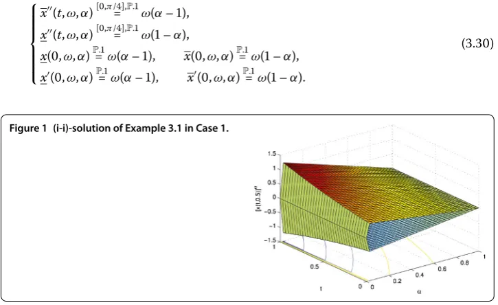
Clearly,xandD,Hgxare (i)-differentiable. Hence, there is an (i-i)-solution in this case. This solution is shown in Figure .
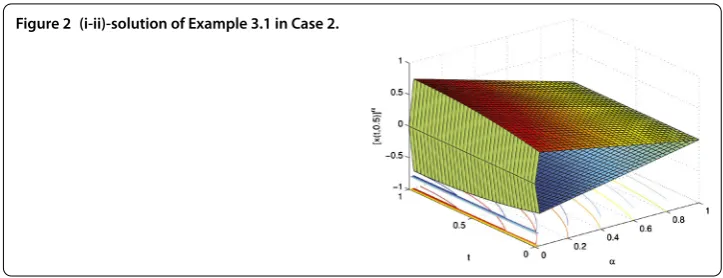
Case: From (.), we have
⎧ ⎪ ⎪ ⎪ ⎪ ⎨ ⎪ ⎪ ⎪ ⎪ ⎩
x(t,ω,α)[,π/],= P.ω(α– ),
x(t,ω,α)[,π/],= P.ω( –α),
x(,ω,α)P=.ω(α– ), x(,ω,α)P=.ω( –α),
x(,ω,α)P=.ω(α– ), x(,ω,α)P=.ω( –α).
(.)
Figure 2 (i-ii)-solution of Example 3.1 in Case 2.
By solving (.), we get
x(t,ω)α=
ω(α– ) +ω(α– )t+ω( –α)t
,ω( –α) +ω( –α)t+
ω(α– )t
.
Clearly, x is (i)-differentiable and D,Hgx is (ii)-differentiable. Hence, there is an (i-ii)-solution in this case. This (i-ii)-solution is shown in Figure .
Case: From (.), we obtain
⎧ ⎪ ⎪ ⎪ ⎪ ⎨ ⎪ ⎪ ⎪ ⎪ ⎩
x(t,ω,α)[,π/],= P.ω(α– ),
x(t,ω,α)[,π/],= P.ω( –α),
x(,ω,α)P=.ω(α– ), x(,ω,α)P=.ω( –α),
x(,ω,α)P=.ω( –α), x(,ω,α)P=.ω(α– ).
(.)
By solving (.), we get
x(t,ω)α=
ω(α– ) +ω( –α)t+ω( –α)t
,ω( –α) +ω(α– )t+
ω(α– )t
.
Sincexis not (ii)-differentiable, there is no (ii-i)-solution in this case.
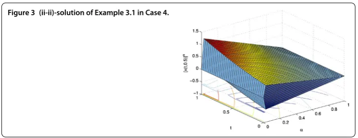
Case: From (.), we have
⎧ ⎪ ⎪ ⎪ ⎪ ⎨ ⎪ ⎪ ⎪ ⎪ ⎩
x(t,ω,α)[,π/],= P.ω(α– ),
x(t,ω,α)[,π/],= P.ω( –α),
x(,ω,α)P=.ω(α– ), x(,ω,α)P=.ω( –α),
x(,ω,α)P=.ω( –α), x(,ω,α)P=.ω(α– ).
(.)
By solving (.), we have
x(t,ω)α=
ω(α– ) +ω( –α)t+ω(α– )t
,ω( –α) +ω(α– )t+
ω( –α)t
.
Figure 3 (ii-ii)-solution of Example 3.1 in Case 4.
Example . Let = (, ), F-Borel σ-field of subsets of , P-Lebesgue measure on (,F). Let us consider the following second-order random fuzzy differential equa-tion:
D,Hgx(t,ω) +x(t,ω)[,π/],=P.(,ω, ω),
x(,ω)P= (–. ω, ,ω), (.)
D,Hgx(,ω)P= (–. ω, ,ω).
Case: From (.), we get
⎧ ⎪ ⎪ ⎪ ⎪ ⎨ ⎪ ⎪ ⎪ ⎪ ⎩
x(t,ω,α) +x(t,ω,α)[,π/],= P.αω,
x(t,ω,α) +x(t,ω,α)[,π/],= P.ω( –α),
x(,ω,α)P=.ω(α– ), x(,ω,α)P=.ω( –α),
x(,ω,α)P=.ω(α– ), x(,ω,α)P=.ω( –α).
(.)
By solving (.), we obtain
x(t,ω)α=ωα( +sint) –ω(sint+cost),ω( –α)( +sint) –ω(sint+cost).
SinceD,Hgxis not (i)-differentiable, there is no solution in this case.
Case: From (.), we have
⎧ ⎪ ⎪ ⎪ ⎪ ⎨ ⎪ ⎪ ⎪ ⎪ ⎩
x(t,ω,α) +x(t,ω,α)[,π/],= P.αω,
x(t,ω,α) +x(t,ω,α)[,π/],= P.ω( –α),
x(,ω,α)P=.ω(α– ), x(,ω,α)P=.ω( –α),
x(,ω,α)P=.ω(α– ), x(,ω,α)P=.ω( –α).
(.)
By solving (.), we get
x(t,ω)α=ωα( +sinht) –ω(sinht+cost),ω( –α)( +sinht) –ω(sinht+cost).
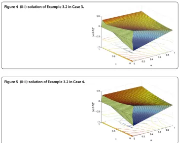
Figure 4 (ii-i)-solution of Example 3.2 in Case 3.
Figure 5 (ii-ii)-solution of Example 3.2 in Case 4.
Case: From (.), we obtain ⎧
⎪ ⎪ ⎪ ⎪ ⎨ ⎪ ⎪ ⎪ ⎪ ⎩
x(t,ω,α) +x(t,ω,α)[,π/],= P.αω,
x(t,ω,α) +x(t,ω,α)[,π/],= P.ω( –α),
x(,ω,α)P=.ω(α– ), x(,ω,α)P=.ω( –α),
x(,ω,α)P=.ω( –α), x(,ω,α)P=.ω(α– ).
(.)
By solving (.), we get
x(t,ω)α=ωα( –sinht) +ω(sinht–cost),ω( –α)( –sinht) +ω(sinht–cost).
Notice that, in this case, sincexis (ii)-differentiable andD,Hgxis (i)-differentiable, such a solution is acceptable. This solution is shown in Figure .
Case: From (.), we have ⎧
⎪ ⎪ ⎪ ⎪ ⎨ ⎪ ⎪ ⎪ ⎪ ⎩
x(t,ω,α) +x(t,ω,α)[,π/],= P.αω,
x(t,ω,α) +x(t,ω,α)[,π/],= P.ω( –α),
x(,ω,α)P=.ω(α– ), x(,ω,α)P=.ω(α– ),
x(,ω,α)P=.ω(α– ), x(,ω,α)P=.ω(α– ).
(.)
By solving (.), we have
x(t,ω)α=ωα( –sint) +ω(sint–cost),ω( –α)( –sint) +ω(sint–cost).
4 Conclusions
In this paper, we discussed the local existence and uniqueness results for the second-order random fuzzy differential equations. Under Lipschitz conditions we obtain the existence and uniqueness theorems of solution for SRFDE. In future work on SRFDEs, we would like to study the local and global existence and uniqueness results of solutions for second-order random fuzzy differential equation under weaker conditions.
Competing interests
The authors declare that they have no competing interests. Authors’ contributions
Each of the authors contributed to each part of the work equally and read and proved the final version of the manuscript. Author details
1Division of Computational Mathematics and Engineering, Institute for Computational Science, Ton Duc Thang University,
Ho Chi Minh City, Vietnam.2Faculty of Mathematical Economics, Banking University, Ho Chi Minh City, Vietnam.
Acknowledgements
The authors would like to express their gratitude to Prof. Vasile Lupulescu, Dr. Ngo Van Hoa (Researcher at Ton Duc Thang University) and the anonymous referees for their helpful comments and suggestions, which have greatly improved the paper.
Received: 31 July 2015 Accepted: 26 November 2015
References
1. Barros, LC, Bassanezi, RC, Tonelli, PA: Fuzzy modeling in population dynamics. Ecol. Model.128, 27-33 (2000) 2. Buckley, JJ, Feuring, T: Fuzzy differential equations. Fuzzy Sets Syst.110, 43-54 (2000)
3. Chang, SSL, Zadeh, L: On fuzzy mapping and control. IEEE Trans. Syst. Man Cybern.2, 30-34 (1972) 4. Dubois, D, Prade, H: Towards fuzzy differential calculus. Fuzzy Sets Syst.8, 225-233 (1982) 5. Zadeh, LA: Fuzzy sets. Inf. Control8, 338-353 (1965)
6. Puri, ML, Ralescu, DA: Differential for fuzzy function. J. Math. Anal. Appl.91, 552-558 (1983) 7. Kaleva, O: Fuzzy differential equations. Fuzzy Sets Syst.24, 301-317 (1987)
8. Wu, C, Song, S: Existence theorem to the Cauchy problem of fuzzy differential equations under compactness-type conditions. Inf. Sci.108, 123-134 (1998)
9. Wu, C, Song, S, Lee, ES: Approximate solutions, existence, and uniqueness of the Cauchy problem of fuzzy differential equations. J. Math. Anal. Appl.202, 629-644 (1996)
10. Song, S, Wu, C: Existence and uniqueness of solutions to Cauchy problem of fuzzy differential equations. Fuzzy Sets Syst.110, 55-67 (2000)
11. Lupulescu, V: Initial value problem for fuzzy differential equations under dissipative conditions. Inf. Sci.178, 4523-4533 (2008)
12. Lakshmikantham, V, Mohapatra, RN: Theory of Fuzzy Differential Equations and Inclusions. Taylor & Francis, London (2003)
13. Lakshmikantham, V, Leela, S: Fuzzy differential systems and the new concept of stability. Nonlinear Dyn. Syst. Theory
1, 111-119 (2001)
14. Mizukoshi, MT, Barros, LC, Chalco-Cano, Y, Roman-Flores, H, Bassanezi, RC: Fuzzy differential equations and the extension principle. Inf. Sci.177, 3627-3635 (2007)
15. Chen, M, Han, C: Some topological properties of solutions to fuzzy differential systems. Inf. Sci.197, 207-214 (2012) 16. Xue, XP, Fu, YQ: On the structure of solutions for fuzzy initial value problem. Fuzzy Sets Syst.157, 212-222 (2006) 17. Lupulescu, V: On a class of fuzzy functional differential equations. Fuzzy Sets Syst.160, 1547-1562 (2009) 18. Malinowski, MT: On random fuzzy differential equations. Fuzzy Sets Syst.160(21), 3152-3165 (2009)
19. Prakash, P: Existence of solutions of fuzzy neutral differential equations in Banach spaces. Dyn. Syst. Appl.14, 407-417 (2005)
20. Agarwal, RP, Lakshmikantham, V, Nieto, JJ: On the concept of solution for fractional differential equations with uncertainty. Nonlinear Anal. TMA72, 2859-2862 (2010)
21. Allahviranloo, T, Salahshour, S, Abbasbandy, S: Solving fuzzy fractional differential equations by fuzzy Laplace transforms. Commun. Nonlinear Sci. Numer. Simul.17, 1372-1381 (2012)
22. Bede, B: A note on ‘Two-point boundary value problems associated with non-linear fuzzy differential equations’. Fuzzy Sets Syst.157, 986-989 (2006)
23. Bede, B, Gal, SG: Generalizations of the differentiability of fuzzy-number-valued functions with applications to fuzzy differential equations. Fuzzy Sets Syst.151, 581-599 (2005)
24. Bede, B, Rudas, IJ, Bencsik, AL: First order linear fuzzy differential equations under generalized differentiability. Inf. Sci.
177, 1648-1662 (2007)
25. Bede, B, Stefanini, L: Generalized differentiability of fuzzy-valued functions. Fuzzy Sets Syst.230, 119-141 (2013) 26. Stefanini, L, Bede, B: Generalized Hukuhara differentiability of interval-valued functions and interval differential
equations. Nonlinear Anal. TMA71, 1311-1328 (2009)
28. Nieto, JJ, Rodríguez-López, R: Bounded solutions for fuzzy differential and integral equations. Chaos Solitons Fractals
27, 1376-1386 (2006)
29. Malinowski, MT: Random fuzzy differential equations under generalized Lipschitz condition. Nonlinear Anal., Real World Appl.13, 860-881 (2012)
30. Malinowski, MT: Existence theorems for solutions to random fuzzy differential equations. Nonlinear Anal. TMA73, 1515-1532 (2010)
31. Nieto, JJ, Khastan, A, Ivaz, K: Numerical solution of fuzzy differential equations under generalized differentiability. Nonlinear Anal. Hybrid Syst.3, 700-707 (2009)
32. Allahviranloo, T, Abbasbandy, S, Ahmady, N, Ahmady, E: Improved predictor corrector method for solving fuzzy initial value problems. Inf. Sci.179, 945-955 (2009)
33. Allahviranloo, T, Abbasbandy, S, Salahshour, S, Hakimzadeh, A: A new method for solving fuzzy linear differential equations. Computing92(2), 181-197 (2011)
34. Allahviranloo, T, Abbasbandy, S, Sedaghatfar, O, Darabi, P: A new method for solving fuzzy integro-differential equation under generalized differentiability. Neural Comput. Appl.21, 191-196 (2012)
35. Salahshour, S, Allahviranloo, T: Applications of fuzzy Laplace transforms. Soft Comput.17, 145-158 (2013) 36. Khastan, A, Nieto, JJ, Rodríguez-López, R: Variation of constant formula for first order fuzzy differential equations.
Fuzzy Sets Syst.177, 20-33 (2011)
37. Hoa, NV, Phu, ND: Fuzzy functional integro-differential equations under generalized H-differentiability. J. Intell. Fuzzy Syst.26, 2073-2085 (2014)
38. Vu, H, Dong, LS, Hoa, NV: Random fuzzy functional integro-differential equations under generalized Hukuhara differentiability. J. Intell. Fuzzy Syst.27, 1491-1506 (2014)
39. Vu, H, Hoa, NV, Phu, ND: The local existence of solutions for random fuzzy integro-differential equations under generalized H-differentiability. J. Intell. Fuzzy Syst.26, 2701-2717 (2014)
40. Dong, LS, Vu, H, Phu, ND: The formulas of the solution for linear-order random fuzzy differential equations. J. Intell. Fuzzy Syst.28, 795-807 (2015)
41. Puri, ML, Ralescu, DA: Fuzzy random variables. J. Math. Anal. Appl.114, 409-422 (1986) 42. Kwakernaak, H: Fuzzy random variables. Part I: definitions and theorems. Inf. Sci.15, 1-29 (1978) 43. Kruse, R, Meyer, KD: Statistics with Vague Data. Kluwer Academic, Dordrecht (1987)
44. Klement, EP, Puri, ML, Ralescu, DA: Limit theorems for fuzzy random variables. Proc. R. Soc. Lond. A407, 171-182 (1986)
45. Colubi, A, Domínguez-Menchero, JS, López-Díaz, M, Ralescu, DA: ADE[0, 1] representation of random upper
semicontinuous functions. Proc. Am. Math. Soc.130, 3237-3242 (2002)
46. Terán Agraz, P: On Borel measurability and large deviations for fuzzy random variables. Fuzzy Sets Syst.157, 2558-2568 (2006)
47. López-Díaz, M, Ralescu, DA: Tools for fuzzy random variables: embeddings and measurabilities. Comput. Stat. Data Anal.51, 109-114 (2006)
48. Puri, ML, Ralescu, DA: The concept of normality for fuzzy random variables. Ann. Probab.13, 1373-1379 (1985) 49. Fei, W: Existence and uniqueness of solution for fuzzy random differential equations with non-Lipschitz coefficients.
Inf. Sci.177, 4329-4337 (2007)
50. Malinowski, MT: Interval differential equations with a second type Hukuhara derivative. Appl. Math. Lett.24, 2118-2123 (2011)
51. Allahviranloo, T, Kiani, NA, Barkhordari, M: Toward the existence and uniqueness of solutions of second-order fuzzy differential equations. Inf. Sci.179, 1207-1215 (2009)
52. Lakshmikantham, V, Gnana Bhaskar, T, Vasundhara Devi, J: Theory of Set Differential Equations in a Metric Space. Cambridge Scientific Publishers, Cambridge (2006)
53. Nguyen, HT: A note on the extension principle for fuzzy sets. J. Math. Anal. Appl.64, 369-380 (1978) 54. Kaleva, O: The Peano theorem for fuzzy differential equations revisited. Fuzzy Sets Syst.98, 147-148 (1998) 55. Chalco-Cano, Y, Román-Flores, H: Comparation between some approaches to solve fuzzy differential equations.
Fuzzy Sets Syst.160, 1517-1527 (2009)