A new kind of parallel finite difference method for the quanto option pricing model

(1)

R E S E A R C H

Open Access

A new kind of parallel ﬁnite difference

method for the quanto option pricing model

Xiaozhong Yang, Lifei Wu

*

_{and Yuying Shi}

*_{Correspondence:}

[email protected]

School of Mathematics and Physics, North China Electric Power University, Beijing, 102206, China

Abstract

The quanto option pricing model is an important financial derivatives pricing model; it is a two-dimensional Black-Scholes (B-S) equation with a mixed derivative term. The research of its numerical solutions has theoretical value and practical application significance. An alternating band Crank-Nicolson (ABdC-N) difference scheme for solving the quanto options pricing model was constructed. It is constituted of the classical implicit scheme, the explicit scheme and the Crank-Nicolson scheme, it has the following advantages: parallelism, high precision, and unconditional stability. Numerical experiments and theoretical analysis all show that ABdC-N scheme can be used to solve the quanto options pricing problems effectively.

Keywords: quanto options pricing model; alternating band Crank-Nicolson (ABdC-N) scheme; stability; parallel computing; numerical experiments

1 Introduction

The multi-asset options pricing model (the multi-dimensional Black-Scholes equation) is a famous financial mathematics basic model; its numerical solutions had played a signif-icant role in promoting a lot of financial derivatives pricing methods. Therefore, the nu-merical solutions have attracted more and more attention from applied mathematicians and economists. With the rapid development of multi-core and cluster technology, paral-lel algorithms have become one of the mainstream technologies improving the numerical calculation efficiency. The research of parallel numerical difference methods for solving a multi-asset options pricing problem has basic scientific significance. This is so because the option pricing has higher time requirements from the need of practical application. Therefore, over the past  years an efficient numerical solution of the multi-asset options pricing model has been the focus of academic research [].

A quanto option is a kind of multi-asset option, the two-dimensional Black-Scholes (D B-S) equation of the quanto option is [–]

∂V ∂t +

 

S_σ_∂

_V

∂S 

+ ρσσSS

∂V ∂S∂S

+σ_S_∂

_V

∂S 

– (r–q)S

∂V ∂S

– (r–q)

∂V ∂S

+rV= ,

q=r–r+q+σσρ, q=r. ()

(2)

Here, we assume an American investor buys a Nikkei index call option.Vis the price of the quanto option (dollar),Sis the price of foreign risk asset (yen),Sis the exchange rate

of the foreign currency against the domestic one (dollar),ris the domestic interest rate

without risk,ris the foreign rate without risk,σis the volatility ofS,σis the volatility

ofS,ρis the correlation coeﬃcient, andqis the dividend.

This equation has the analytical solutions:

V(S,S,t) =

e–r(T–t)

π(T–t)σσ

 –ρ

× _∞



_∞



(η–K)+

η

exp

σ_α_– ρσσαα+σα

σ_σ_( –ρ₍_T_–_t₎₎

dηdη,

α=ln

S

η

+

r–q–ρσσ–

α 



(T–t),

α=ln

S

η

+

r–r–

α_ 

(T–t).

Here,Kis the strike price of the options (yen),Tis the due date of the options (year). The analytical solution is very complex, difficult to quickly solve, so numerical solutions were usually used to compute option pricing models in the real financial market, for exam-ple, the Monte-Carlo method, the binary tree method, and the finite difference method, etc.[, ]. The considered computing speed and accuracy, and the finite difference method was usually used in the real financial market.

In recent years, the study of finite difference methods for solving the dual currency tion pricing model has made a lot of progress. An implicit scheme for the multi-asset op-tion pricing model had been made by Gilliet al.(), but a calculation of this scheme was relatively complex; one needed to solve algebra equations which contained a large tridiagonal block matrix []. Khaliqet al.() had given a kind of difference method for solving the D B-S equation []; the method needs to use the penalty function approach. So the method was difficult on using parallel computing on a computer. Yang and Zhou () had put forward a rapid AOS difference method of quanto option pricing model [], but the calculation accuracy of the method is not ideal, because the error of its mixed derivative term is not ideal. In addition, most of those schemes had applied serial calcula-tion. When the computing grid points or dimension of equation required is large, a higher order algebraic equationAx=bshould be solved. The efficiency of the calculation process is not ideal, and it is difficult to meet the requirements of the options as regards time.

(3)

and we have second-order convergence. Yuan () has put forward a parallel diﬀerence scheme with second-order accuracy and unconditional stability for a nonlinear parabolic system [].

For the quanto option pricing model (D B-S equation), we used the classical implicit scheme, the explicit scheme, and the Crank-Nicolson scheme, constructed a parallel dif-ference scheme-alternating band Crank-Nicolson (ABdC-N) scheme, which is uncondi-tionally stable, and which is close to second-order accuracy. Numerical experiments show that the method is eﬀective.

2 ABdC-N difference scheme

2.1 Initial-boundary value condition of 2D B-S equation

In order to solve the equation of the quanto option pricing model, the initial condition and boundary condition meeting () will be given in this section. In theory, the solving area of this equation is

(S,S,t)| <S<∞,  <S<∞,t∈[,T] .

But in the actual transaction, the price of the underlying asset will not always appear to be zero or inﬁnity. Therefore, the ﬁnancial institution provides a small enough valueSmin

(Smin> ) as the lower bound and a large enough valueSmax(Smax> ) as the upper bound

for it. Then the pricing problem can be solved in the bounded area

=(S,S,t)|Smin<S<Smax,Smin<S<Smax,t∈[,T] .

Assume that the foreign option is the call option, then construct the initial and boundary conditions for (). For the reason that the option pricing is a backward problem, the initial condition is

V(S,S,T) =S·max{S–K, }.

The boundary conditions are

V(Smin,S,t) = , V(Smax,S,t) = ,

V(S,Smin,t) = , V(S,Smax,t) = .

In order to solve (), we can substitute its variable as follows [, ]:

x=lnS, y=lnS, τ=T–t.

Then this pricing model will be transformed into the initial-boundary value problem of a partial diﬀerential equation with constant coeﬃcients:

∂V ∂τ –

 

σ_∂

_V

∂x + ρσσ

∂V ∂x∂y+σ

 

∂V ∂y

–

r–q–

σ 



∂V ∂x –

r–q–

σ 



∂V

(4)

q=r–r+q+σσρ, q=r. () 2.2 Construction of the ABdC-N scheme

Letx,y,τ be the steps ofx,y, andτ, respectively. Here,x= (lnSmax–lnSmin)/m,

y= (lnSmax–lnSmin)/n,τ=T/nt,m,n,ntare positive integers.xi=lnSmin+ix,

yj=lnSmin+jy,τk=kτ,i= , , . . . ,m,j= , , . . . ,n,k= , , . . . ,nt. For convenience, leth=x=y. We useV_ik_,_jto denote the solution of () at point (xi,yj,τk).

We introduce the following notation:

δxVik,j=

A classical diﬀerence scheme of () is as follows:

τV_ik_,_j=

The above scheme can be written as

θ–aVik–,+j–aVik,j+––bVik+,+j–bVik,j++–cRVik,j+

Here, () is called the universal diﬀerence scheme (θ-scheme).

(5)

implicit scheme, which has unconditional stability. Whenθ= ., () is a classical Crank-Nicolson scheme, which is of second-order accuracy and has unconditional stability. But

the implicit scheme’s and the C-N scheme’s computing times are longer.

The design of ABdC-N is as follows.

Assume the value of thekth time layerVk

i,j(i= , , . . . ,m– ) is known, the value of the

i,j . At the remaining points, we apply the classical C-N scheme (θ= .) to calculateV_ik_,_j+. Whenkis an odd number, at pointxi,j(i=I,I, . . . ,Is), we apply the implicit scheme (θ= ) to calculateV_ik_,_j+; at pointxi,j(i=I,I, . . . ,Is–), we

apply the explicit scheme (θ= ) to calculateVk+

i,j . At the remaining points, we apply the classical C-N scheme (θ= .) to calculateV_ik_,_j+.

(6)

gm–=

3 Existence and uniqueness of the ABdC-N scheme solution Assume the valueVk

i,jof thekth time layer is known, the valueVik,j+of thek+ th time layer waits for calculating. From the ABdC-N scheme (), the matrix equation for calculating the value of thek+ th time layer is

(E+DG)Vk+= (E–DG)Vk+gk/. ()

The coeﬃcient matrix isE+DG. From the expression ofG, we can see thatGis a

diago-nally dominant matrix. SoE+DGis also a diagonally dominant matrix. In other words,

E+DGis a nonsingular matrix. Therefore, formally () has a unique solution. Similarly,

applying the ABdC-N scheme () to calculate the value of thek+ th time layer, the co-eﬃcient matrixE+DGof this matrix equation is also a nonsingular matrix. Therefore,

this matrix equation of thek+ th time layer has a unique solution. Based on the above analysis, we will get the following theorem.

Theorem  The ABdC-N scheme () for solving the quanto option pricing model is uniquely solvable.

4 Stability and convergence of the ABdC-N scheme

The stability and convergence of the ABdC-N scheme for solving the quanto option pric-ing model will be analyzed in this section. The growth matrix of the ABdC-N scheme () is

(7)

For discussing the stability of the ABdC-N scheme, we need to introduce the Kellogg lemma [].

Lemma  Ifρ> and C+CT_{is a non-negative}₍_{or positive}₎_matrix_,_then₍_ρ_E₊_C₎–_exists_,

and(ρE–C)(ρE+C)– ≤.

Lemma  DG,DG in the growth matrix of the ABdC-N scheme for solving the quanto

option pricing model are non-negative matrices.

Proof If DG, DGmeet the requirement thatDG+ (DG)T,DG+ (DG)T are

non-negative matrices, and Lemma  is correct. Therefore, we only need to prove DG+

(DG)T,DG+ (DG)Tare non-negative matrices. We have

DG+ (DG)T=D

G+GT

=D

⎛ ⎜ ⎜ ⎜ ⎜ ⎝

Am– –(a+b)E

–(a+b)E Am– –(a+b)E

. .. . .. . ..

–(a+b)E Am–

⎞ ⎟ ⎟ ⎟ ⎟ ⎠,

Am–= 

⎛ ⎜ ⎜ ⎜ ⎜ ⎝

α –a–b

–a–b α –a–b

. .. . .. . .. –a–b α

⎞ ⎟ ⎟ ⎟ ⎟ ⎠.

Form the deﬁnition ofa,b,a,b,α, it is obvious thatDG+ (DG)Tis a diagonally

domi-nant matrix and the diagonal elements ofDG+ (DG)Tare non-negative real numbers. In

other words,DG+ (DG)Tis a non-negative matrix. Similarly, we see thatDG+ (DG)T

is also a non-negative matrix. Therefore,DGandDGare non-negative matrices.

Note

M= (E+DG)T(E+DG)–= (E–DG)(E+DG)–(E–DG)(E+DG)–.

From Lemma , we know thatAGandAGare non-negative matrices. We can apply

Lemma  to get the following inequality easily:

(E–DiG)(E+DiG)–_≤, i= , .

Then we getρ(M) =ρ(M)≤ T≤. Therefore, we get the following theorem.

Theorem  The ABdC-N scheme()for solving the quanto option pricing model is uncon-ditionally stable.

Due to the Lax theorem [], we can get a corollary.

(8)

5 Accuracy of the ABdC-N scheme

First, the accuracy of universal difference scheme () for solving the quanto option pricing model will be analyzed in this section. The universal difference scheme will be expanded as the Taylor series at the point (xi,yj,τk). Then we can get the truncation errorT(τ,h), Crank-Nicolson scheme at this time. The truncation error is of second order in time and space. Whenθ= , , the truncation is of first order in time and second order of space.

From the construction of the ABdC-N scheme, we take inside points without interior boundary points as ‘interior point’. Because the ABdC-N scheme () is applied to the C-N scheme at the interior point, the truncation error of the interior point is of second order. The truncation error of interior boundary points will be analyzed in the following. The ABdC-N scheme () alternatively applies the classical explicit scheme and the implicit scheme at the interior boundary points.

The two classical schemes approximate the analytical solution from either side, respec-tively. It had been proved that the numerical solution of the classical explicit schemeθ=  is greater than the analytical solution, and the numerical solution of the classical implicit schemeθ =  is less than the analytical solution. Therefore, alternatively applying them can improve the calculation accuracy. For example, the truncation error of the ‘Explicit-Implicit scheme’ or the ‘‘Explicit-Implicit-Explicit scheme’ is of second order in time and space, and unconditionally stable. In the ABdC-N scheme () for solving the quanto option pricing model is alternatively applied the classical explicit and the implicit scheme at the interior boundary point; then the truncation error of interior boundary point also can achieve a second order.

Theorem  The truncation error of the ABdC-N scheme()for solving the quanto option pricing model is O(τ+h_).

(9)

6 Numerical experiments

Numerical experiments will be done in Matlab a, based on Intel core i- CPU@.GHz. The comparison is between the ABdC-N scheme and the classical C-N scheme, referring to computing accuracy and computing time.

Example We consider an American investor buying a Nikkei index call option.

Assum-ing the current price of Nikkei is , yen, the dividend rate of the Nikkei is ., the volatility of the Nikkei is ., the exchange rate of Japanese yen against dollar is ., the volatility of the exchange rate is ., the correlation coeﬃcient is ., the risk-free rates of American and Japan are . and ., respectively. The strike price of an option is , yen. We consider the deadline of the option to be one year ( months), and the ﬁnal exchange rate is the spot exchange rate.

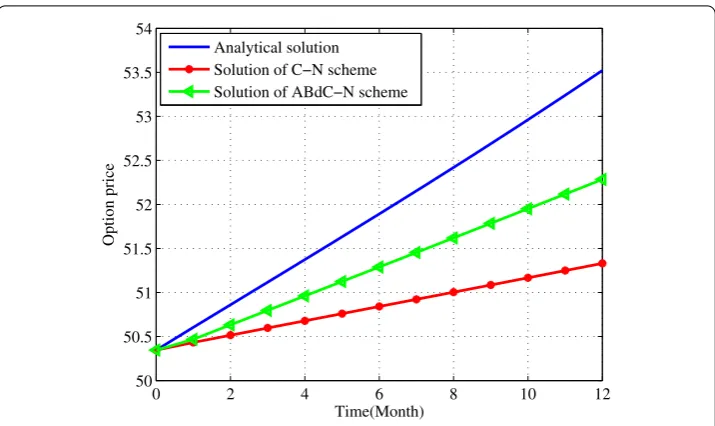
In terms of the computation accuracy, from Table , we can see that the accuracy of numerical solution of the ABdC-N scheme is high, and is close to the classical C-N scheme. By comparing numerically the ABdC-N scheme and the C-N scheme from Table , the relative error of the numerical solution of ABdC-N is .%, and the relative error of the classical C-N scheme is .%. The numerical result of the ABdC-N scheme is closer to the analytical solution than the classical C-N scheme.

Next we will analyze the root mean square error (RSME) of the ABdC-N scheme and C-N scheme. The solutions of the diﬀerence scheme are denoted asu¯i,j. The analytical solution is denoted asui,j. The deﬁnition of RSME is as follows:

RSME=

M

i=

N

j=(ui,j–u¯i,j)

M∗N .

The ratio of RSME (RRSME) is deﬁned as

RRSME=RSME h .

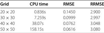
From Tables  and , the RSMEs of the ABdC-N scheme and the C-N scheme are be-coming smaller and smaller with mesh grid reﬁnement. The RSME of the ABdC-N scheme is smaller than the classical C-N scheme’s. This shows that ABdC-N scheme is better than the classical C-N scheme in terms of computation accuracy. The RRSMEs of the ABdC-N

Table 1 Comparison of analytical and numerical solution

Scheme 12 months Relative error CPU time

Analytical solution 53.521809 -

-Classical C-N scheme 51.331487 4.09% 158.157s

ABdC-N scheme 52.284465 2.49% 18.037s

Table 2 Error analysis of classical C-N scheme

Grid CPU time RMSE RRMSE

20×20 0.836s 0.1450 2.900

30×30 7.259s 0.0999 2.997

40×40 38.07s 0.0762 3.048

(10)

Table 3 Error analysis of the ABdC-N scheme

Grid CPU time RMSE RRMSE

20×20 1.410s 0.0795 1.590

30×30 2.095s 0.0547 1.641

40×40 5.649s 0.0417 1.668

50×50 18.307s 0.0336 1.680

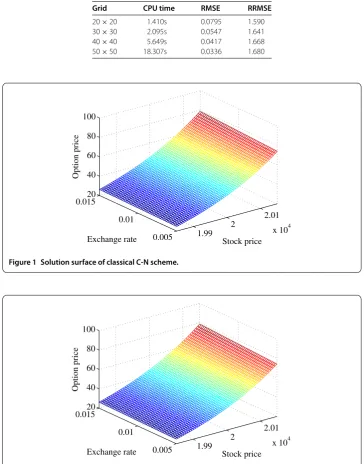
Figure 1 Solution surface of classical C-N scheme.

Figure 2 Solution surface of the ABdC-N scheme.

scheme are near . for each grid. The RRSMEs of the C-N scheme are near . for each grid. This shows that the ABdC-N scheme and the C-N scheme have better stability.

(11)

Figure 3 Comparison of analytical and numerical solution.

In terms of computation time, from Tables , , and , the computing time of the ABdC-N scheme of the quanto option has a big advantage compared with the classical C-N scheme (except grid ×). When the number of grid points is smaller, the impact of the data communication on the cycle can greatly reduce the computation eﬃciency. So when the grid is ×, the CPU time of the C-N scheme is smaller than the ABdC-N scheme. The computing time (CPU time) of the ABdC-N scheme is .%, .%, .% of the C-N scheme for grids ×, ×, ×, respectively. When the number of grid points is larger, the advantages of parallel computing of the ABdC-N scheme are obviously superior. The computation time of the ABdC-N scheme can save about % compared with the classical C-N scheme for grid ×. Therefore, the ABdC-N scheme can be more eﬀective to solve option pricing problems than the classical C-N scheme.

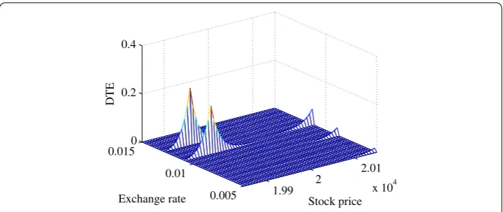
In order to better compare the accuracy of the ABdC-N scheme with the classical C-N scheme, we will analyze the distribution of the diﬀerence total energy (DTE) at space grid points for grid ×. Taking the numerical solutionu¯ of the classical C-N scheme as the control solution, we take the numerical solutionuof the ABdC-N scheme as a pertur-bation solution. The deﬁnition of DTE is as follows []:

DTE(i,j) =  

nt

k=

¯

uk_i_,_j–uk_i_,_j.

From Figure , the scope of DTE is ∼.. In other words, the numerical solution of the ABdC-N is very close to the C-N scheme. The value of DTE is relatively large in three lines of the y axis (exchange rate). The three lines are inside the boundary points, the ABdC-N scheme alternatively applies the classical explicit scheme and the implicit scheme which are of ﬁrst order accuracy. Therefore, the value of DTE is relatively large within the three lines.

(12)

Figure 4 Distribution of DTE at space grid points.

7 Conclusion

An alternating band Crank-Nicolson (ABdC-N) difference scheme for solving the quanto options pricing model (D B-S equation) has been constructed. The computing accuracy, stability, and convergence of the ABdC-N scheme have been analyzed. The result of the numerical experiments is consistent with the theoretical analysis. The ABdC-N scheme has an ideal computing accuracy and computing efficiency, and it can be more effective to solve the quanto options pricing problems.

Competing interests

The authors declare that they have no competing interests.

Authors’ contributions

All authors contributed equally and signiﬁcantly in writing this article. All authors read and approved the ﬁnal manuscript.

Acknowledgements

This work is sponsored by the project National Science Foundation of China (No. 11371135, 11271126), the Fundamental Research Funds for the Central Universities (Nos. 13QN30, 2014ZZD10).

Received: 16 June 2015 Accepted: 23 September 2015 References

1. Kwork, YK: Mathematical Models of Financial Derivatives, 2nd edn. The World Book Publishing Company, Beijing (2011)

2. Jiang, LS: Mathematical Modeling and Methods of Option Pricing, 2nd edn. Higher Education Press, Beijing (2008) (in Chinese)

3. Li, YQ, Huang, LH: Quanto Option and Delay Option Pricing Research. Hunan Unniversity Press, Changsha (2011) (in Chinese)

4. Gilli, M, Kellezi, E, Pauletto, G: Solving ﬁnite diﬀerence schemes arising in trivariate option pricing. J. Econ. Dyn. Control26(9-10), 1499-1515 (2002)

5. Khaliq, AQM Voss, DA, Kazmi, K: Adaptiveθ-methods for pricing American options. J. Comput. Appl. Math.222(1), 210-227 (2008)

6. Yang, XZ, Zhou, GX: A kind of accelerated AOS diﬀerence schemes for dual currency option pricing model. Int. J. Inf. Syst. Sci.7(2-3), 369-378 (2011)

7. Evans, DJ, Abdullah, ARB: Group explicit methods for parabolic equations. J. Comput. Math.14, 73-105 (1983) 8. Zhang, BL: Alternating segment explicit-implicit methods for diﬀusion equation. J. Numer. Method Comput. Appl.4,

245-253 (1991)

9. Wang, WQ: Diﬀerence schemes wit intrinsic parallelism for the KdV equation. Acta Math. Appl. Sin.29(6), 995-1003 (2006) (in Chinese)

10. Sheng, ZQ, Yuan, GW, Hang, XD: Unconditional stability of parallel diﬀerence schemes with second order accuracy for parabolic equation. Appl. Math. Comput.184, 1015-1031 (2007)

11. Yuan, GW, Sheng, ZQ: The unconditional stability of parallel diﬀerence with second order convergence for nonlinear parabolic system. J. Partial Diﬀer. Equ.20, 45-64 (2007)

12. Yang, XZ, Liu, YG, Wang, GH: A study on a new kind of universal diﬀerence schemes for solving black-Scholes equation. Int. J. Inf. Syst. Sci.3(2), 251-260 (2007)

(13)

14. Zhang, SC: Finite Diﬀerence Numerical Calculation for Parabolic Equation with Boundary Condition. Science Press, Beijing (2010) (in Chinese)