Applying the Transfer Learning Techniques on Classification Model A Brief Survey

Applying the Transfer Learning Techniques on Classification Model – A

Brief Survey

Nisha Sathyan

_{VR. Nagarajan}

1,2

_{Assistant Professor}

1,2

_{Department of Computer Science & Engineering}

1

_{Chinmaya College of Arts, Commerce & Science, Tripunithura, Kochi, Pin 682301, India}

2

_{Sree Narayana Guru College, Coimbatore - 641 105, India}

Abstract— The major conjecture in traditional machine learning process is both the training data and test data. The future test data must have same dissemination and it should contain same feature space. This identical conjecture may not be applicable to many real world applications. The identical conjecture might be infringed when a new data emerges from another new domain while the older domain has their own labelled data. One of the domains may contain classification task and ample training data may persist in another domain and also the last-mentioned data may exist in different feature space and different data distribution concept is followed. The method of labelling is more expensive and the process of transfer learning can be applied to become cost effective. The learning performance can be improved and the labelling efforts can be reduced by transfer learning concept. The Boosted Transfer Learning (TrAdaBoost) concept is established and the users are permitted to exploit only a few amounts of recently labelled data to hold the old data to produce the accurate classification model for the new data with high quality. The Boosted Transfer Learning is compared with inductive transfer learning, transductive transfer learning and unsupervised transfer learning to prove that TrAdaBoost effectively transfers the knowledge from old to new data.

Key words: Machine Learning, Boosted Transfer Learning, Inductive Transfer Learning, Transductive Transfer Learning, Data Mining

I. INTRODUCTION

The techniques such as classification, regression and clustering are the notable technologies achieved in Data Mining as well as Machine Learning. The concept of machine learning is possible in two cases: i.e. both training and test data are taken from similar feature space and distribution. The conjecture in classification learning method is to have an identical data distribution. This classification method goes wrong when this identical data distribution doesn’t takes place. When there is a change in data distribution, then most of the factual models needs to be reconstructed from expunge utilizing the new training data [1]. Reorganizing the training data is costly and reconstructing turns to be impossible. The effort and requisite to reorganize the training data can be effectively reduced by transfer learning method.

Most of the applications such as web mining, this type of learning may not be possible since there is a frequent change in the web content. The web page classification model gets antiquated due to the frequent changes and labeling the new data is very expensive. Even though, few data items can be reused when the training data gets antiquated. The new data classifier can be trained by the knowledge learnt from the training data. Those data can be found by recruiting a few

amounts of labeled recent data that helps to select the features of old data and this procedure is called same distribution of training data. The training data is said to be different distribution when the antiquated training data comes under the diverse distribution of new data.

Consider the indoor Wi-Fi localization problem by which the user’s exact location can be determined from formerly collected Wi-Fi information. In large scale environment, measuring the Wi-Fi data in a building is expensive because large amount of Wi-Fi data signal needs to be labeled. The building localization model constructed in one period of time may affect the performance in another time period and hence the estimation effort needs to be reduced. The efforts taken to measure the Wi-Fi data can be reduced by adapting the building model constructed at one period of time (source data) to new model at another period of time (target data).

In order to adapt this localization model, a transfer learning technique must be implemented to transfer the knowledge from old data to new data. The survey is done by comparing the three transfer learning techniques: inductive transfer learning, transductive transfer learning and boosted transfer learning and the boosted transfer learning model is examined to be cost effective. The boosted transfer learning TrAdaBoost is based on Probability Approximately Correct (PAC) method. The motive of this method is to refine the different distribution training data that is extremely different from same data distribution by instinctively modifying the weights of training data. The rest of the different data distribution is the supplementary training data that helps to boost the effect of learned model even though the same distribution data is inefficient [15]. The boosted transfer learning framework model is developed to produce this type of high performance simple learning model.

The remaining sections are categorized as follows: section 2 demonstrates the work related to transfer learning; section 3 gives the overview of transfer learning; section 4 demonstrates about the existing methods – inductive, transductive and unsupervised transfer learning methods; section 5 demonstrates the proposed model – boosted transfer learning; section 6 deals with result analysis based on data sets; section 7 gives the conclusion about transfer learning.

II. RELATED WORK

another domain in 1987. The transfer would prevail as the large method and procedure, but the learning task should have similar characteristics like transfer task. The generalization concept could support the similarity in terms of learning and transfer tasks. The generalization of transfer tasks should be similar to learning task and this was found by H. Al-Mubaid and S. A. Umair.

Huang, J., Smola, A., Gretton, A., Borgwardt, K. M., & Sch¨olkopf, B in 2007 established the concept of generalization that permits the people to act to the new cases because of the similar tasks associated with the familiar features [6]. Gagne in 1965 recommended the lateral and vertical transfer process. The skills can be applied to another type of domain which has the same level of difficulties and the transfer is called lateral transfer. The same set of skills can be applied to other domain which contains more complex features. Baldwin and Ford organized the works regarding training inputs that includes training features, design and task; training outputs includes knowledge transfer required during training in the year 1988. The solution is provided for the available transfer task and future enhancements. Rouillier and Goldstein in 1993 defined the transfer as situational cues and consequences.

Schmidhuber in 1994 introduced the concept of “how to learn”, Thrun and Mitchell in 1995 introduced the concept “learning one more thing” and Caruana in 1997 introduced “multi task learning” in 1997 [3]. Ben David and Schuller in 2003 have given the proof for multi task learning. Wu and Dietterich in 2004 invented the image classification algorithm that uses both insufficient training data and poor quality auxiliary data. Some enhancements have been done by auxiliary data. But they failed to provide quantitative study on auxiliary data. Liao et al introduced the active learning to improve the learning with auxiliary data in 2005.

Rosenstein et al in 2005 proposed the new idea on transfer learning using Naive Bayes approach using auxiliary data to improve its performance. Zadrozy in 2004 found the associated task learning in sample selection bias system or co-variate shift method where the labeling is done for same data distribution. The sample selection bias method was corrected by Heckman in 1979. The concept of spam filtering domain was coordinated with corrected sample selection bias by Dudik et al in 2006.

III. OVERVIEW OF TRANSFER LEARNING

The statistical models used in machine learning and data mining algorithms anticipate the future data based on the trained labeled or unlabelled data. Using the labeled and unlabelled data, the classification problem can be minimized by semi supervised classification method. The previously obtained knowledge can be intelligently applied to resolve the new issues or to afford new solutions to the problem. The concept of transfer learning is termed as “life long learning” because it preserves and reuse the previously gained knowledge.

The transfer learning became familiar in the year 1995 and it has different names like incremental/cumulative learning, knowledge transfer, inductive transfer, knowledge based learning and multi task learning. In these methods, multi task learning is closely connected to transfer learning

concept where the multiple tasks are learnt simultaneously. Based on the common characteristics, the individual task gets benefited.

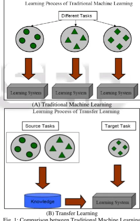
The new mission about transfer learning was given by Information on Processing Technology of DARPA (Defense Advanced Research Projects Agency). The mission was developed to admit and implement the well-read knowledge from old tasks to new tasks. The knowledge applied to the target domain is the knowledge obtained from the source domain. The multi-task learning method gives more importance to both target domain and source domain whereas transfer learning is attentive only towards target domain. The comparison between traditional machine learning and transfer learning methods are illustrated in figure 1. In traditional machine learning, the knowledge is obtained from the deleted data while the knowledge is obtained from source domain and applied to target domain in transfer learning.

(A) Traditional Machine Learning

(B) Transfer Learning

Fig. 1: Comparison between Traditional Machine Learning and Transfer Learning

A. Notations Used in Transfer Learning

The diverse feature space or different probability distribution occurs when the two domains are from different areas.

The domain is specified as D = {A, P (A)} and the task attribute includes the label space feature B and its predicate function is denoted as f (.) i.e. U = {B, f (.)}. The value of U is the knowledge obtained from the trained data but it is not observed anywhere. It also contains the sets {ai, bi} where ai ϵ A and bi ϵ B. The predicate function f (.) determines the label and f (a) of the new instance a [8]. The probability of f (a) is denoted as P (b|a). Consider the example for classifying the document where B is the group of labels which tells true value, false value for binary feature classification task and bi holds the true or false.

Consider the scenario, where the source domain is given by DS and its target is denoted as DT. The domain source data is specified as DS = {(aS1, bS1), ……(aSn, bSn)} and aSi ϵ AS and bSi ϵ BS where AS is the data instance and BS is the class label. The term vectors are DS and its class labels are true or false in classification of the document [14]. The target data is represented as DT = {(aT1, bT1), ……(aTn, bTn)} and aTi ϵ AT and bSi ϵ BT is the output.

In this approach, the data set is taken and compared with different transfer learning methods like inductive transfer learning, transductive transfer learning, unsupervised transfer learning and boosted transfer learning and the analysis shows that the errors are less in boosted transfer learning compared to others.

IV. EXISTING MODELS

A. Inductive Transfer Learning

In this type of transfer learning, the target and source domain are different. There is no necessity of having same source and target domain attributes. The labeled training data specified in the target domain are needed to instigate the predicate function fT (.) and depending on different labeled and unlabelled source data it can be used in the target domain. When the large amount of labeled data is available in the source, then the multi task learning method is considered because the inductive transfer learning method is equal to multi task learning concept.

The inductive transfer learning concentrates only on the target domain by performing knowledge transfer from source domain whereas the multi task transfers the knowledge between the task and source domains simultaneously to achieve high performance. When the labeled source domain data are not available, self-taught learning method is considered since the inductive transfer learning performs the actions of self-taught learning method [7]. The space labeled between source and target tasks are different in self-taught learning method which indicated that the back side data of the source task cannot be applied straightly. This method is also assumed to be the same where the labeled source data seems to be not available.

In the inductive transfer learning, the source task and learning task are denoted by DS and TS. Similarly the target domain and its learning task are denoted by DT and TT. The learning task of the predictive function fT (.) in target domain DT can be enhanced by considering the knowledge obtained in both DS and TS and also the condition says that TS is not equal to TT.

The inductive transfer learning approach is called as instance transfer approach because the labeled data in target task are focused and the source tasks are not reused straightly. The inductive transfer learning helps to identify the exact feature representations of different types of source task. The supervised learning approach is used to create the feature data for the large amount of available labeled data. It is connected to multi task learning and also called as common feature learning method. The unsupervised learning approach is used to create the feature data for the available unlabelled source data [1].

The supervised learning approach is equivalent to multi task learning method. The low dimensional data representation is conveyed across the corresponding tasks. The errors occurred in the classification or regression approach can be minimized in the learned representation of new task. The sparse coding technique is applied in unsupervised learning approach to use high level attributes [13]. The first step is to learn the vectors of high level features on the source task and the second step is to construct the optimization algorithm on the target task to transfer the high level features. The discriminative algorithms can be related to their labels to enhance the classification or regression techniques in the target task. But this type of method is not applicable for utilizing the high level attributes of source task in the target task.

The transfer approaches related to inductive transfer learning is the related tasks of individual models that share the features of hyper parameters. The multi task learning method includes the concept of regularization and hierarchical Bayesian framework. The multi task learning focuses on source and target task learning whereas the transfer learning concept focuses on enhancing the performance of target data by using the source data [2]. In multi task learning method, the weights calculated for the loss functions are appeared to be the same for both source and target data. In transfer learning approach, the weights calculated for the loss function are appeared to be different for diverse domains. Hence the large amount of weight value is assigned to the loss function to attain high performance in target data.

B. Transductive Transfer Learning

The transductive transfer learning was invented by Arnold where the source and target tasks are similar but the domain appears to be different. The source and the target data domain are dissimilar in transductive transfer learning but the task data appear in the source and target are the same. A huge amount of labeled data is available and the labeled data are not available in target domain [15]. The transductive transfer learning technique occurs where the feature space is not the same in target and source domain and it is denoted as AS is not equal to AT. The second type is the feature space are the same in source and target domain i.e. AS = AT, but the probability distributions of source data are not the same where P (AS) is not equal to P (AT).

the test data are needed at training and the learned data cannot be reused for the new data. In the process of transfer learning, the task data can be similar but there exists an unlabelled data in the target domain.

The notations used in transductive transfer learning are:  DS  Source domain

 TS  Associated learning task  DT  Target domain

 TT  Associated learning task

 FT (.)  Predicate function of target can be improved by the knowledge obtained in DS and TS.

Where DS is not equal to DT and TS = TT condition holds and few of the unlabelled data of target domain may occur during the training time. This concept is termed as “domain adaptation” method since it is similar to traditional machine learning that effectively utilizes the unlabelled data for learning [4]. The unlabelled target domain data is taken for the purpose of classification. The definition states that the similar source and target data are used to accommodate the learned predictive function and target domain and this is applicable with the help of unlabelled data of target domain [12].

The steps in transductive transfer learning are:  Setting the sampling based method

 Assess the empirical risk minimization problem

 The optimal model is learnt for reducing the expected risk in target domain

 The model is learnt from the domain source data because of the unavailability of labeled data in the domain target and solved by optimization

When source domain data is not equal to target domain data then the optimization can be revised with the ability of high generalization attributes in target domain

Hence the overall performance can be greatly improved by combining the features of source data with target data. The quality is generated by a trained source classification. Still this method may have computational burden and this can be overcome by boosted transfer learning process with minimum errors [11].

C. Unsupervised Transfer Learning

In unsupervised transfer learning method, the labeled data are not seen in both source and target domain during training. The methods like self-taught clustering (STC) and transfer discriminative analysis are initiated to reduce the dimensionality transfer and transfer clustering [7].

The notations used in unsupervised transfer learning are:  DS  Source domain

 TS  Associated learning task  DT  Target domain

 TT  Associated learning task

 FT (.)  the unsupervised transfer learning applies the knowledge in both DS and TS to improve the predicate function of target domain.

 The condition holds: TS is not equal to TT and BS and BT are not noticeable

The steps involved in unsupervised transfer learning are:  Clustering is performed by combining both the

unlabelled data of target domain with the source domain

 The common feature space data are learnt to perform clustering and can be solved by optimization

 Apply the transferred discriminative analysis to reduce the dimensionality transfer

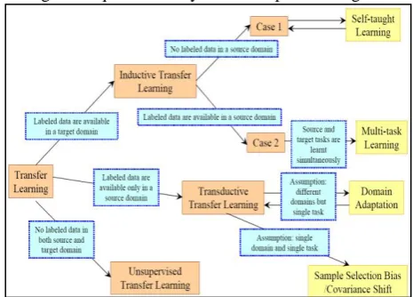
The advantage of unsupervised learning is to perform clustering in order to reduce the dimensions [15]. Still the error ration is higher and it can be resolved by boosted transfer learning. The different types of transfer learning techniques are analyzed and depicted in figure 2.

Fig. 2: Types of Transfer Learning Models

V. METHODOLOGY – BOOSTED TRANSFER LEARNING

The transfer learning can be enabled by using some parts of labeled training data with the same distribution to construct the classification model and the model is called as same distribution training data, but it remains insufficient for constructing the classification model. The test data and the training data distribution are different because they are old model and it is called as different distribution training data. The amount of different distribution data is very large and the classification model cannot be used to test the data.

Here, boosted transfer learning framework is adopted called as TrAdaBoost. The classifier model and the weak learner’s accuracy can be adjusted deliberately. AdaBoost concept is equivalent to traditional machine learning methods by making the conjecture that training and test data are identical [9]. AdaBoost is extended to transfer learning and this is assigned to the same distribution training data to frame the foundation of the model. In the case of different distribution, when the distributed changes made by the learned data are not correctly forecasted and the most different data are conflicted to same distribution data. The steps involved in boosted transfer learning methods are:  When the different distribution training data is not

predicted correctly and the collected data may have dispute with same distribution data.

 The training weight and its effect can be reduced by increasing the weights.

 The different distribution data which are not similar to same distribution data may have influence on the learning process.

that are not equivalent to same distribution have lower weights.

 By performing the step 4, the weight loss and error prediction can be determined. The TrAdaBoost helps to optimize the weight loss as well as to minimize the error and the algorithm is shown in figure 3.

Fig. 3: Steps in TrAdaBoost

The TrAdaBoost minimizes the error ratio on the same distribution data and the weight loss can be reduced in different distribution data.

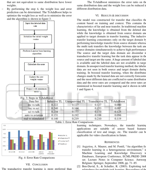
VI. RESULTS & DISCUSSION

The model was constructed for transfer that classifies the content based on training and context. This contains the characteristics of far and near transfer. In traditional machine learning, the knowledge is obtained from the deleted data while the knowledge is obtained from source domain and applied to target domain in transfer learning. The inductive transfer learning concentrates only on the target domain by performing knowledge transfer from source domain whereas the multi task transfers the knowledge between the task and source domains simultaneously to achieve high performance. The source and the target data domain are dissimilar in transductive transfer learning but the task data appear in the source and target are the same. A huge amount of labeled data is available and the labeled data are not available in target domain. In unsupervised transfer learning method, the labeled data are not seen in both source and target domain during training. In boosted transfer learning, when the distributed changes made by the learned data are not correctly forecasted and the most different data are conflicted to same distribution data and the error rates are compared and the error rates are minimized in boosted transfer learning and it shown in table 1 and figure 4.

Data Set Inductive TL Unsupervised TL Transductive TL TrAdaBoost

rec vs talk 0.222 0.127 0.127 0.080

rec vs sci 0.240 0.164 0.153 0.097

sci vs talk 0.234 0.177 0.173 0.125

auto vs aviation 0.131 0.192 0.188 0.096

real vs stimulated 0.140 0.219 0.210 0.119

Table 1: Error Rate Comparisons

Fig. 4: Error Rate Comparisons

VII. CONCLUSION

The transductive transfer learning is more preferred than inductive and supervised transfer learning. The basic classifier model is boosted by performing knowledge transfer from same distribution to different distribution attributes. The additional training data are called as different distribution data for analyzing the labeled same distribution data. The analysis shows that the boosted transfer learning model first classifies the same distribution training data and then prefer different distribution data as supplementary data. Hence the error rates are smaller when compared to other transfer

learning techniques. Nowadays, the transfer learning applications are suitable of sensor based features, classification of text and image, etc. The transfer can be applicable for video classification in future.

REFERENCES

[1] Argyriou, A. Maurer, and M. Pontil, “An algorithm for transfer learning in a heterogeneous environment,” in Machine Learning and Knowledge Discovery in Databases, European Conference, ECML/PKDD 2008, ser. Lecture Notes in Computer Science. Antwerp, Belgium: Springer, September 2008, pp. 71–85. [2] Ben-David, S., & Schuller, R. (2003). Exploiting task

relatedness for multiple task learning. Proceedings of the Sixteenth Annual Conference on Learning Theory. [3] Caruana, R. (1997). Multitask learning. Machine

Learning, 28(1), 41–75.

[4] Daum´eIII, H., & Marcu, D. (2006). Domain adaptation for statistical classifiers. Journal of Artificial Intelligence Research, 26, 101–126.

and Data Engineering, vol. 18, no. 9, pp. 1156–1165, 2006.

[6] Huang, J., Smola, A., Gretton, A., Borgwardt, K. M., & Sch¨olkopf, B. (2007). Correcting sample selection bias by unlabeled data. In Advances in neural information processing systems 19.

[7] R. Raina, A. Battle, H. Lee, B. Packer, and A. Y. Ng, “Self-taught learning: Transfer learning from unlabeled data,” in Proceedings of the 24th International Conference on Machine Learning, Corvalis, Oregon, USA, June 2007, pp. 759–766.

[8] Rosenstein, M. T., Marx, Z., Kaelbling, L. P., & Dietterich, T. G. (2005). To transfer or not to transfer. Proceedings of NIPS 2005 Workshop on Inductive Transfer: 10 Years Later.

[9] Schapire, R. E. (1999). A brief introduction to boosting. Proceedings of the Sixteenth International Joint Conference on Artificial Intelligence.

[10]Schmidhuber, J. (1994). On learning how to learn learning strategies (Technical Report FKI-198-94). [11]Shimodaira, H. (2000). Improving predictive inference

under covariate shift by weighting the log-likelihood function. Journal of Statistical Planning and Inference, 90, 227–244.

[12]T. Joachims, “Transductive inference for text classification using support vector machines,” in Proceedings of Sixteenth International Conference on Machine Learning, 1999, pp. 825–830.

[13]Thrun, S., & Mitchell, T. M. (1995). Learning one more thing. Proceedings of the Fourteenth International Joint Conference on Artificial Intelligence.

[14]X. Ling, W. Dai, G.-R. Xue, Q. Yang, and Y. Yu, “Spectral domaintransfer learning,” in Proceedings of the 14th ACM SIGKDD International Conference on Knowledge Discovery and Data Mining. Las Vegas, Nevada: ACM, August 2008, pp. 488–496