Volume 2008, Article ID 675048,12pages doi:10.1155/2008/675048
Research Article
Robust OFDM Timing Synchronisation in Multipath Channels
C. Williams,1, 2S. McLaughlin,3and M. A. Beach1
1Centre for Communications Research, Bristol University, Woodland Road, Bristol, BS8 1UB, UK 2Hayes, Fujitsu Laboratories of Europe, London, UB4 8FE, UK
3Institute for Digital Communications, University of Edinburgh, Mayfield Road, Edinburgh, EH9 3JL, UK
Correspondence should be addressed to C. Williams,[email protected]
Received 11 September 2007; Revised 19 February 2008; Accepted 21 April 2008
Recommended by Athina Petropulu
This paper addresses pre-FFT synchronisation for orthogonal frequency division multiplex (OFDM) under varying multipath conditions. To ensure the most efficient data transmission possible, there should be no constraints on how much of the cyclic prefix (CP) is occupied by intersymbol interference (ISI). Here a solution for timing synchronisation is proposed, that is, robust even when the strongest multipath components are delayed relative to the first arriving paths. In this situation, existing methods perform poorly, whereas the solution proposed uses the derivative of the correlation function and is less sensitive to the channel impulse response. In this paper, synchronisation of a DVB single-frequency network is investigated. A refinement is proposed that uses heuristic rules based on the maxima of the correlation and derivative functions to further reduce the estimate variance. The technique has relevance to broadcast, OFDMA, and WLAN applications, and simulations are presented which compare the method with existing approaches.
Copyright © 2008 C. Williams et al. This is an open access article distributed under the Creative Commons Attribution License, which permits unrestricted use, distribution, and reproduction in any medium, provided the original work is properly cited.
1. INTRODUCTION
Orthogonal frequency division multiplex (OFDM) is widely used in or proposed for a number of communication appli-cations, including wireless LAN [1] and digital broadcast systems [2, 3], this is due to its inherent robustness to intersymbol interference (ISI) as a consequence of employing a cyclic prefix (CP). For adequate performance, an ISI free symbol must be presented to the FFT process, and thus timing estimation is critical. Additionally, fine frequency estimation is required to minimise intercarrier interference (ICI). Such algorithms need to be robust to varying mul-tipath conditions, which could include transmissions from multiple transmitters, as in a broadcast single frequency network (SFN). A number of synchronisation algorithms have been proposed in the literature [4–16], many of which exploit the correlation properties of the cyclic prefix. How-ever, the ability of these methods to provide accurate timing and frequency estimation in a wide range of multipath channels is limited. Further, to ensure the most efficient data transmission possible, there should be no constraints on how much of the cyclic prefix is occupied by ISI. In this paper, synchronisation of the terrestrial digital video
broadcast system (DVB) [2] is investigated. This system uses a cyclic prefix but does not include dedicated training symbols. Further, the application of interest is to provide a solution of mobile terminals, and so operation at vehicular speeds is required.
A motivation for the work presented in this paper was to develop a low-complexity solution to pre-FFT synchro-nisation for multimode terminals. A multimode terminal communicates with a number of networks, though not necessarily simultaneously. To minimise acquisition time when switching between networks, maintaining a coarse synchronisation to each network is desirable. This requires the algorithm to be suitable for a wide range of channels (including mobile channels), different air interface param-eters and not reliant on post-FFT processing. This would allow a terminal to maintain synchronisation to different systems (potentially with different air interfaces) and reduce the requirement for more complex FFT processing.
The method presented here is an extension of [5]. This paper offers a detailed theoretic foundation for the method, and provides analysis of the performance by simulation. Further, a new variance reducing enhancement is described based on a set of heuristic rules using the peaks of the correlation and derivative functions. The results are com-pared against the basic correlation approach, and a second derivative approach.
In the following section of this paper, the basic notation used throughout is introduced. Issues relating to OFDM timing estimation and previously proposed techniques are then reviewed in the following section, and derivative-based methods are described. The comparative performance of the methods is then presented, followed by a description of further enhancements to the first derivative method. Finally, a summary of the paper with conclusions and potential wider applications is presented.
2. NOTATION
An OFDM symbol consists of 2M + 1 complex sinusoids modulated by complex modulation values{X(j)}, wherejis the subcarrier index. The output OFDM symbol of lengthN
samples, with time indexk, is given by theN-point complex modulation sequence:
x(k)= 1
N
M
j=−M
X(j)ej2πk j/N,
k=0, 1, 2,. . .,N−1; N≥2M+ 1.
(1)
This process is efficiently carried out using an inverse DFT. The individual sinusoids are orthogonal on the useful interval of the symbol. For a sample interval of Ts, the
separation of subcarriers is 1/(N·Ts), and the useful period
of the symbol isTu=N·Ts.
To mitigate against intersymbol interference (ISI), a cyclic prefix (CP), or guard interval, of Ng samples, is
inserted before each symbol. The guard interval of Tg =
Ng·Ts is chosen to exceed the largest expected multipath
delay. The periodic nature of the DFT is exploited by making the guard interval a replica of the last Ng symbols of the
symbol. The transmitted symbol thus consists ofNS=N+Ng
samples.
In the multipath channel case,P + 1 is the number of multipath components, the path amplitudes area(n),θis the received signal timing offset,ε is the frequency offset, and n(k) is additive channel noise. Whens(k) is the transmitted signal, the received signal is
r(k)=
P
p=0
s(k−θ−p)a(p)ej2πε(k−p)/N+n(k). (2)
3. REVIEW OF OFDM SYNCHRONISATION
3.1. Pre-FFT synchronisation
Synchronisation algorithms for OFDM can be divided into two classes, pre-FFT and post-FFT. The primary goal of
pre-FFT processing is to provide a symbol of data to the FFT process, such that ISI and ICI are minimised, otherwise the output from the FFT will be degraded. Thus pre-FFT processing must provide coarse timing alignment (FFT win-dow alignment) and fractional frequency offset correction. Post-FFT processing, commonly using pilot information, can provide the fine timing correction estimates, sample fre-quency correction, and integer frefre-quency offset corrections. For pre-FFT synchronisation, the structure of the symbol needs to be exploited, either using the CP [4], inserting a short repeating sequence [6] or dedicated training symbols [7,8]. Also, to be applicable to a wide range of systems, the synchronisation algorithm must be able to work well with short guard intervals. However, since both methods produce synchronisation estimates using a correlation process, the same form of estimator can be used in both cases.
For timing estimation, a timing point at the start of the useful symbol interval is the ideal. Where the maximum delay spread isτmax, the timing point can be advanced into
the CP by up toTg−τmax. However, any delay of the timing
point will introduce ISI.
Exploiting the redundancy introduced by the CP to estimate time and frequency parameters is most commonly performed by averaging the correlation between the CP and the end of the useful symbol, as analysed by van de Beek et al. [4]. For timing estimation in additive white Gaussian noise (AWGN), the maximum likelihood function consists of a summed correlation term and an energy correction term (E) which is a function of signal-to-noise ratio (SNR), as shown in (3) (see [4] for details). In this paper,γ(m) in (3) below will be called the correlation function,
γ(m)=
m+Ng−1
k=m
r(k)r∗(k+N) +E,
E=ρ.1 2
m+Ng−1
k=m
r(k)2
+r(k+N)2,
ρ= 1
1 +SNR−1,
(3)
where r(k) is the received signal. A two-step optimisation process first estimates the timing offset (assuming zero-frequency offset) based on the peak of γ(m), and then the frequency offset is calculated based on the phase shift between the CP and the end of the symbol. In dispersive environments, the performance is degraded since the corre-lation will include ISI. This limits the accuracy of the timing estimation, and so this method is good for coarse acquisition in some environments, but other processing is required for fine tracking. ISI corruption is more severe for short guard intervals, where the proportion of ISI free CP is limited. Some previously reported proposals to improve performance of CP-based techniques include the following.
(2) Alternatively, the length of the correlation window can be increased to include a greater proportion of the multipath energy [13].
(3) Exponentially weight the summation bywm−k, where m is the trial offset as used in (3), and k is the summation index [9]. This reduces the impact of ISI on the assumption that the strongest multipaths have the shortest delay. By choosing the weighting factor
wso thatw =1−2−M, multiplication is reduced to
simple shift and adds.
(4) To prevent ISI from the following symbol when the timing estimate is in error, and positive, the actual DFT window position can be advanced by an amount (such as half the CP interval). Clearly, if the advance is too great there is an increased probability of ISI from the preceding symbol.
These all place constraints on the ISI characteristics which is undesirable.
3.2. Analysis of correlator output in
multipath channels
It is shown in the appendix that the correlation function γ(m) from (3) is a triangular function in AWGN, the ideal timing point is at the peak, and the length of the slopes is the CP interval (Tg).
In multipath, following (2), the output of a correlator is
r(k)r∗(k+m)
Taking expectations, and again assuming i.i.d. symbols and noise samples, nonzero terms only arise fromm=0,N,N−
p,N+ p. Except for very long multipath delays, the latter two terms are unlikely to occur, and ignoring the trivial autocorrelation, only them=Nterms are of interest. Thus,
E{r(k)r∗(k+N)}
In evaluating the expectation operation, not all multipath terms will contribute due to the i.i.d. symbols assumption. Defineσ2
s as the signal variance, K as the symbol number,
andastart offset for each symbol asK=K(N+Ng) samples.
Three cases are considered as follows.
(1) All multipath components are due to current symbol, and so all terms are included in the summation:
Er(k)r∗(k+N) =σ2
(2) Longer delayed multipath components generated by previous symbol do not contribute:
Er(k)r∗(k+N) =σ2
(3) Shortest delayed multipath components generated by next symbol do not contribute:
Er(k)r∗(k+N) =σ2
Otherwise, the expectation is zero. Consider now the contribution to the expectation by a single multipath component,φ, denotedEr(k,φ). Again, the three cases apply
for nonzero expectations to arise the following equations:
Er(k,φ)=σs2e−j2πεa(φ)
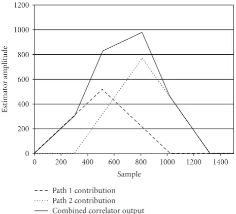
This demonstrates that the contribution from each multi-path component needs a triangular function, with a peak delayed byθ+φ. Therefore, from linearity of the expectation functions, the combined expectation is the summation of triangular functions of each multipath component, delayed bypand weighted by|a(p)|2. Thus forPpaths,
In multipath channels, the peak ofγP(m) does not necessarily
point to the position of the first arriving path, as demon-strated inFigure 1. In this situation, ISI will occur due to the delayed timing estimate.
1200 1000 800 600 400 200 0
0 200 400 600 800 1000 1200 1400
Estimat
o
r
amplitude
Sample Path 1 contribution Path 2 contribution Combined correlator output
Figure1: Summed correlation function for two-path channel.
3.3. Correlation detection for multipath channels
For dispersive channels, timing estimation methods that detect the leading edge of the correlator output may provide improved performance. A straightforward way to do this is to set a threshold, and detect the crossing of this threshold [14]. For complex channels and for a time-varying SNR, the amplitude of the correlation characteristic will change in time, so the threshold needs to be set relative to this peak. In a purely AWGN channel, as the threshold is decreased, the chosen timing point will move forward in direct proportion (e.g., for a threshold of 75% of the peak correlation, the timing point will be advanced by 25% of the guard interval length). Thus, for the AWGN channel compensation is straightforward. However, for a dispersive channel, the relationship is dependent on the multipath characteristic which will not be known in advance.
Huang et al. [15] noted that within the ISI-free portion of the CP, the phase of the correlator output would be constant (the offset is proportion to the frequency offset). Outside this interval, the phase would be a random variable. It was proposed to detect the change from constant value to random value as an estimate for the timing point. The offset in the phase measurement provides an estimate for the frequency offset. This method shows good performance but requires a long averaging period, is sensitive to frequency offset, and requires that a portion of the CP is ISI free, otherwise the method fails. An alternative solution is just to form the scalar subtraction separated by the useful symbol interval [11] and to sum over a suitable number of samples. However, this method does not work with frequency offset because the phase rotation corrupts the subtraction. In this case, frequency correction would be required before timing estimation, which has difficulties. Palin and Rinne [16] notes that for most channels the correlation function will not
change significantly from symbol to symbol. Consequently, carrying out a second correlation with the correlation outputs from adjacent symbols would give a lower variance estimate. This is indeed the case; however, the mean value is similar to that from the basic correlator method.
Synchronisation based on the signal’s statistical prop-erties has also been proposed. Subspace processing based on second-order statistics has been described in [17], which has good performance in multipath channels, but the complexity is high, as so is the quantity of samples required. With so many samples, the mobility supported is low. Cyclostationary properties can also be exploited [18,19], but these also require processing over many symbols with a static channel and a high SNR may be needed. In order to have cyclostationary features, suitable structure, such as pulse shaping [19], needs to exist.
3.4. Derivative methods
Figure 1has shown that peak detection from the correlation function can give a high-estimation error in multipath environments. Each multipath component adds its own weighted and delayed triangular functionγi(m), rising and
falling over periods of Ng samples. When the maximum
multipath delay is less thanNg, (for the period corresponding
to the rising edge of the first multipath component, 0 to 512 inFigure 1), the functionsγi(m) of the other components are
being added in, and all are rising. After the peak of the first component, the functionγ1(m) starts to fall, and the other
functions will also in turn stop increasing and fall at a point according to the path delay. Therefore up to the peak of the first component, the slope of the combined correlator output γP(m) is monotonically increasing (no noise). After the peak
position of the first component, the slope ofγP(m), though
possibly positive, starts to decrease. Therefore the ideal timing point (when the multipath is bounded byNg) is the
point at which the derivative of the functionγP(m) starts to
decrease, regardless of the channel power delay profile. The dashed line in Figure 2demonstrates this. Alternatively, in the ideal case, this point is a negative-going zero crossing of the second derivative of the functionγP(m). Both techniques
are investigated.
The method of obtaining timing estimates is now explained, and is illustrated inFigure 3. From (3), for time offsetkand symbol indexK, the correlator output is
γKN+kTs
=
Ng−1
i=0
rKN+kTs
r∗KN+kTs+iTs
.
(13)
15 10 5 0 −5 −10 −15
×102
0 512 1024 1536
Estimat
o
r
amplitude
Sample Combined correlator output Differentiation
Smooth
Figure2: Correlation derivative and smoothed derivative functions
(ideal timing at sample 512).
length over a range of lengths. The estimate of the derivative is thus
dKN+kTs
=γKN+kTs
−γKN+ (k−1)Ts
,
bKN+kTs
=
Ng/2
i=0
dKN+ (k−i)Ts
.
(14)
This smoothed estimate is termed the derivative function. The estimation problem for the first derivative method is to find the point at which this derivative function starts to fall after its peak. In practice, before the derivative function falls, there may be an extended flat portion of this function, and so peak detection alone will result in poor performance. In this work, the falling edge is projected backwards (using a least square (LS) fit), and the position of the intersection with the level of the peak of the derivative function, p(K), is the timing-point estimate. This approach needs to decide which samples to take to form the linear fit. In this investigation, two thresholds are set relative to the derivative peaks,T1%
andT2% , and the samples falling between these points (and
after the peak),β(K), are used. This can be described as
b(KN+kTs)∈β(K) ifT1< b(KN+kTs)< T2,
(KN+kTs)> nP(KN).
(15)
The thresholds depend on the length of the CP, for the short (64-point) CP used here, thresholds of 40% and 95% relative to the derivative function peak have been used. For other applications, these thresholds would require reviewing, for example, for a 512-point CP, thresholds of 60% and 90% were effective.
From the elements of the setβ(K), an LS fit forb=A+Bk is found to give the parametersAandB, hence the estimated timing point for this symbol is given by
nest(K)= p
(K)−A
B . (16)
The estimate based on the second derivative adds a further derivative estimator to that shown inFigure 3, which again uses an averaging filter after a one-point differentiator. In practice, many zero crossings exist due to noise for the second derivative estimate with a single path channel. A minimum after the ideal timing point was evident, and so the timing estimate was chosen to be the zero crossing immediately prior to this minimum. As with the first derivative approach, an LS line fit could be used to smooth the estimate, but for this approach, the benefits are small compared to the additional complexity, and so this has not been included.
The processing described so far provides one timing estimate per symbol. Occasionally, it has been found that synchronisation parameter estimates have a large error, but these are isolated events. Using a median filter, of lengthLM
with outputm(K), is an effective method of removing these spurious results. ForNg of 64 samples (Nis 2048 samples), a
15-point median filter followed by a 16-point FIR filter, more generally of lengthLAwith outputs(K), have been used to
good effect. For longer CPs, shorter filters can be used. The estimate filtering can be summarised as
m(K)=mediannest(K)· · ·nest
K−LM ,
s(K)=
LA−1
l=0
m(K−l). (17)
Thus for the results presented in this paper, each timing estimate is the result of filtering over 16 symbols. Such filtering will reduce the maximum mobility to which the synchronisation algorithm is tolerant, but for the Doppler spreads considered here, these filters do not have a significant effect.
4. PERFORMANCE
For this investigation, the simulations conform to the DVB-T system [2], using the 2k-mode with 16 QAM modulation, and a 64-point CP with virtual subcarriers used. The DVB-T standard allows CP lengths up to 512, the shorter one used here is more challenging for synchronisation algorithms. A channel representative of a single frequency network (SFN) has been used, with two transmitters each having an independent channel response. The DVB-T simulator includes the pilot and signalling structure as defined in [2], including the appropriate PN sequences.
r(k) From ADC
Correlator γ(k)
Differentiate and average (repeated for 2nd derivative)
b(k)
LS fit A,B Sample rate
Get timing estimate by projection
Symbol rate
nest(K) Median filter
Average filter
m(K)
s(K) Timing estimate
Figure3: Block diagram of the timing estimator.
with K-factor of−4.8 dB, and the deterministic component has a relative frequency offset of 0.33 compared to the maximum Doppler frequency (channel UR1 in [20]). The channel is thus parameterised as a function of the relative delay and power of the two SFN components. The channels have independent fading. Unless noted otherwise, standard parameters are 0 dBEb/N0, equal power channels with delay
31 samples (3.4μs). Results for a more complex channel are presented inSection 4.
In the maximum likelihood case, the energy correction term in (2) is a function of the SNR [4], and it is known that this term is important to estimation performance [21]. In practice, taking an assumed SNR of infinity (soρin (3) is equal to 1) does not degrade performance, and this has been done in these investigations.
4.1. Estimation accuracy
The timing estimation error statistics for the Beek and the two derivative algorithms have been investigated. In this paper, the error performance is shown in terms of mean error and standard deviation because representing the error just in terms of a mean square error results in information being lost, since it is not clear whether the error is dominated by the bias of the estimator or the variance. A high Doppler spread of 200 Hz has been used (the subcarrier spacing is 4464 Hz), which equates to 270 km/hr at 800 MHz. Investigations have shown that timing performance is relatively insensitive to Doppler spread up to and beyond this value. Frequency estimation as described above does show a rapidly increasing variance above this frequency. With this Doppler spread, the deterministic component of the channel model is at 66 Hz. As noted in [4], the frequency estimates using the method of [4] are relatively insensitive to timing variations, and investigations have shown the frequency estimation results to be similar for the different timing estimation algorithms. The results presented were generated from 20 frames of data (1380 symbols).
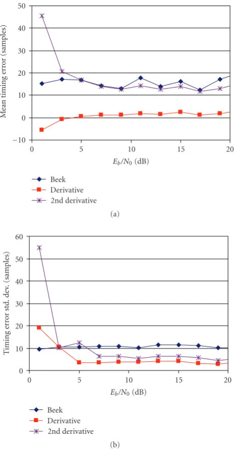
The estimation results are presented in Figures4 to 6.
Figure 4 shows performance as a function of Eb/N0, and
demonstrates that the mean error of the proposed first derivative method is significantly lower than that in the other methods, and the estimate variance is also lower. The inherent bias of the mean and variance of the Beek estimates in relation to the channel delay spread is clearly shown in
Figure 5, whereas the mean of the first derivative method is lower and less dependent on the channel. The variance
of the derivative method increases more rapidly inFigure 5
when the channel response is longer than the CP. Figure 6
shows how the first derivative method biases its estimates towards the first arriving path as the strength of the second path is increased, and the peak variance is reduced compared to the Beek method. These performance plots show how the variance of the first derivative method is typically better than the second derivative method, and the second derivative method has a significantly worse mean timing error. The bias in the mean timing error is channel dependent and so cannot be removed without prior knowledge of the channel, or post-FFT processing. For the channels with a short CP, the difficulty in getting a good second derivative estimate means that estimation using the second derivative does little better than the basic peak detection of the correlation function (Beek method).
4.2. System performance
This section compares the bit error rate performance of the DVB-T system for the Beek method, the first derivative method, and an “ideal” case which uses perfect knowledge of the start of the symbol (first multipath component arrival), so no synchronisation correction is applied. For these simulations, the Doppler spread is 40 Hz (equivalent to 54 km/hr at 800 MHz), so that any equaliser limitations do not affect the results. For these simulations, receiver equal-isation and decoding (convolutional and Reed-Solomon) processes are included. The equaliser linearly interpolates between pilots in the frequency domain only. No post-FFT synchronisation processing has been included (except equalisation), and so the assumption has been made that no integer frequency offset exists. Frequency estimation is based on that described in [4]. For this analysis, the number of frames sent was the minimum of (i) 7 frames (476 symbols) and (ii) the equivalent of 20 times the channel coherence time. A minimum of 50 bit errors was then required, up to a maximum number of transmitted symbols of 10 000.
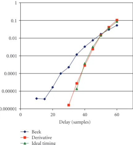
Figures7and8show a comparison as a function ofEb/N0
and delay of the second multipath component, where it is seen that the derivative technique has a performance close to the system with ideal timing estimation, and is better than the peak detection method.
50
Figure4: Timing-error performance comparison as a function of
Eb/N0.
delay spread exceeds the CP length, and so ISI is inevitable. In this case, performance can be improved by delaying the timing point to introduce precursor ISI, but this is more than compensated by the reduction in postcursor ISI. This compensation is channel dependent. The ideal case does not admit precursor ISI (aligns with first multipath component), but the Beek case does. Hence at the extreme case shown on the right of the graph, the delayed timing point from the Beek algorithm improves performance. However, the performance in this parameter region is poor, and is not useful for communications, so is not as relevant in practical scenarios.
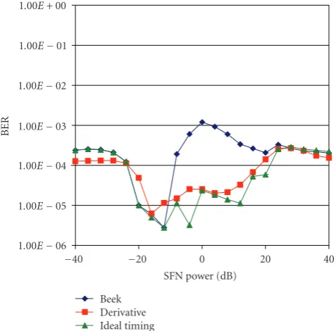
Figure 9shows the effect of changing the relative power of the second transmitter. The improved performance in the
60
Figure5: Timing-error performance comparison as a function of
SFN delay.
transition region, where the two multipath components have similar power, is clear.
To summarise, the derivative technique can provide improvements in system performance, even for short CPs. These benefits are maintained for longer CPs and more com-plex channels, though equaliser performance can become the limiting factor due to the scattered pilot structure of DVB-T.
5. ENHANCEMENTS
35 30 25 20 15 10 5 0 −5 −10
−40 −20 0 20 40
M
ean
timing
er
ro
r
(samples)
SFN scale (dB) Beek
Derivative 2nd derivative
(a) 12
10 8 6 4 2 0
−40 −20 0 20 40
T
im
in
g
er
ro
rs
td
.d
ev
.(
sa
m
p
le
s)
SFN scale (dB) Beek
Derivative 2nd derivative
(b)
Figure6: Timing-error performance comparison as a function of
SFN power.
additional information from the correlation and derivative functions can help to reduce the variance by identifying unlikely estimates, and replacing them with ones more consistent with current information, and past estimates. In particular, we consider the position of the peaks of these functions.
Let each rule be denoted with indexi asRi(tE), where
tE is the time index of estimates (incremented per OFDM
symbol). The value of the limit itself will be denoted with Li(tE). For example, based on the behaviour of the
correlation and derivative functions, the following rules are proposed.
(1) The timing estimate cannot be later than the peak of the correlation function output. Denote this asR1(tE).
1
0.1
0.01
0.001
0.0001
0.00001
5 10 15 20
BER
Eb/N0(dB) Beek
Derivative Ideal timing
Figure7: Error performance as a function ofEb/N0.
1
0.1
0.01
0.001
0.0001
0.00001
0.000001
0 20 40 60
BER
Delay (samples) Beek
Derivative Ideal timing
Figure8: Error performance as a function of SFN delay.
(2) The timing estimate cannot be earlier than the correlation function peak minus the CP length, since the peak will always be within the CP interval. Denote this as R2(tE).
(3) The timing estimate cannot be earlier than the peak of the derivative function, since the timing point is the breakpoint after the peak. Denote this asR3(tE).
Table1: Bug UN2 channel characteristics.
Tap delay (μs) 0 0.33 0.73 1.51 2.16 2.64 3.04 3.32
Tap amplitude (dB) 0 −4.1 −6.7 −10.8 −7.9 −9.6 −10.5 −11.0
1.00E+ 00
1.00E−01
1.00E−02
1.00E−03
1.00E−04
1.00E−05
1.00E−06
−40 −20 0 20 40
BER
SFN power (dB) Beek
Derivative Ideal timing
Figure9: Error performance as a function of SFN power.
with the imposed limits and possibly the previous estimates as well. Three estimation replacement approaches are pro-posed, and have been investigated. Referring to Figure 10, they are as follows.
(1) Hard replacement. When a limitRi(tE) is exceeded,
the estimate is replaced by the limit, that is,B(t) =
Li(tE).
(2) “Before” replacement. Replace by previous input to the estimate filter, that is,B(tE)=B(tE−1).
(3) “After” replacement. Replace by previous output of the estimate filter, that is,B(tE)=C(tE−1).
There may be situations where more than one rule is broken and the results may conflict, for example,R1(tE) andR3(tE).
For this study, the rules were tested in the order presented above. ForR1(tE) andR3(tE) both broken, there is a conflict
sinceR1(tE) wants to delay the estimate, andR3(tE) wants
to advance it. Again with this ordering, the most advanced option is chosen since, as previously discussed, it is preferable to advance the estimate than to delay it.
The DVB-T 2k mode simulation as previously described has been used. While previously a median filter of length 15 and an FIR filter of length 16 were used, shorter filters of lengths 5 and 8, respectively, have also been used. Additionally, the results are presented for an 8-path multipath profile from each transmitter (channel UN2 in
[20]), each with a maximum delay of 31 samples. Table 1
provides the multipath characteristic for this channel. The results show a small increase in mean timing error of a few points when the rules are applied, but the mean timing error shows a flatter characteristic. More significant changes are seen in the standard deviation of the estimation error, and for brevity, only these are shown.
It can be seen fromFigure 11that replacing bad estimates with the last output from the estimate filter gives a consistent improvement in performance. Also shown is the result for the same algorithm with a shorter estimate filter; it is clear that there is only a degradation of a few samples in the standard deviation. Thus for a small loss of performance, much reduced filtering could be employed. Shorter filters will reduce latency through the estimation process and so the estimator can track faster moving channels.
Figure 12shows the benefits when the delay between the multipath clusters is varied. Again, the “after” replacement strategy performs the best, and there is little loss when a shorter filter is employed. Noticeable with the UN2 channel is that, without the rules processing, when the maximum combined delay exceeds the CP length, there is a rapid increase in standard deviation. Which is expected since this breaks one of the assumptions made in the derivation of the derivative method. However, the rule-based processing significantly suppresses this characteristic. It has been noted that over a range of channel conditions, the proposed rules are used in approximately equal proportion, and so including all three is justified.
6. SUMMARY AND CONCLUSIONS
A new multipath-robust OFDM timing estimation technique based on the derivative of the summed correlation function has been proposed and the performance examined for the DVB-T system. Even in the worst case considered of very short CPs, the method has shown to be superior to the peak detection method. In considering complexity, the synchronisation algorithms are dominated by the correlation calculation, and the additional number of multiplications of the derivative and LS fitting are less than 1%. An initial constraint was that the ISI is limited to the guard interval, but with the additional rules based processing, this need not be the case.
From
Figure10: Block diagram for rule processing.
20
Figure11: Performance of rule-based processing as a function ofEb/N0.
25
an additional timing offset correction based on the post-FFT timing estimation. This paper does not include post-post-FFT correction to enable the true performance of the proposed method to be determined.
To compensate for the bias, an advance is required to provide ISI free FFT-windows. Any such advance requires that portion of the CP to be ISI free, and therefore gives a reduction in the effective length of the CP for ISI mitigation. This advance corresponds to 31% for the short CP (64 points), and only 5% of the CP for the long CP (512 points) not shown here. For the short CP, the advance required is in excess of 50 samples for both the Beek and second derivative methods (over 78%). Therefore, this method requires a reduced offset compared to the other techniques examined. In practice, a combination of pre- and post-FFT estimation will reduce the advance required, but the ability of the first derivative method to get good estimates quickly has been demonstrated.
The technique is applicable to a wide range of applica-tions. Although presented as a DVB-T [2] broadcast scenario, it would be effective for any OFDM system with a CP, and with multipath maximum delay bounded by the CP length. In particular, the potential for rapid synchronisation is suitable for DVB-H [22], and the results presented here are directly applicable due to the similarities between the physical layers of these standards. For OFDMA, we need to identify the first arriving user, everyone else will have advanced timing, where the allowable advance depends on the effective multipath delay (i.e., the user relative signal delay and delay spread combined). The effective multipath delay can be controlled using feedback to give coarse frequency and timing alignment [23]. With the reasonable assumption that the signals from each user are independent, and with the maximum effective multipath delay less than the CP length, the combined correlation function is the summation of the individual functions and so the analysis presented here applies.
Similarly, the analysis is unchanged for the repeated symbol method of Schmidl [6], with R segments and NR
samples in each segment (typically R·NR = N +Ng, or
some multiple thereof, e.g., see [1]). Extending the previous correlation in (3) overR·NR/2 will lead to similar analysis,
with the benefits of a longer averaging period, as long as the multipath delay is less thanNRsamples.
Therefore in both these applications, the derivative method will provide enhanced performance.
APPENDIX
In this Appendix, the expectation of the correlator output for an AWGN channel, as developed in [4], is reviewed as a precursor to the generalisation to the multipath case in the main text. Note that in [4], the maximum likelihood (ML) function includes an energy correction term. Since the formulation here does not claim to be an ML solution, and for simplification, the energy correction term is not included. Define the signal index setI{θ,. . .,θNg−1}, which is the set of points in the CP.σ2
nis the noise variance. Where virtual
subcarriers are not used, the pointwise expectation of the
output of the correlator can be considered in the following cases:
∀k∈I:Er(k)r∗(k+m) =
(1)m = 0; E{r(k)r∗(k+m)} = σ2
s + σn2 (zero delay
autocorrelation);
(2)m=N;E{r(k)r∗(k+N)} =σ2
se−j2πε(delay by useful
symbol period);
(3) otherwise;E{r(k)r∗(k+m)} =0.
On the assumption of i.i.d. symbols, the expectation for points not in the setI is zero. The output of the correlator is summed overNg samples, thus
C(k)=
k+Ng
n=k
r(n)r∗(n+N). (A.1)
Taking the expectation, and defining E{r(n)r∗(n+N)} =
D(n),
E{C(k)} =
k+Ng
n=k
D(n),
D=
⎧ ⎨ ⎩
σ2
se−j2πε θ−Ng< k−K< θ+Ng,
0 otherwise.
(A.2)
Thus for the Kth symbol, the expected output of the summation of correlator output is a triangular function.
ACKNOWLEDGMENTS
The work reported in this paper has formed part of the Wireless Enablers area of the Core 3 Research Programme of the Virtual Centre of Excellence in Mobile & Personal Communications, Mobile VCE,http://www.mobilevce.com, whose funding support, including that of EPSRC, is grate-fully acknowledged. Fully detailed technical reports on this research are available to Industrial Members of Mobile VCE.
REFERENCES
[1] IEEE Std 802.11a/D7.0-1999, Part11: wireless LAN medium access control (MAC) and physical layer (PHY) specifications: high speed physical layer in the 5 GHz band.
[2] EN 300 744, “Digital Video Broadcasting (DVB); framing structure, channel coding and modulation for digital terres-trial television (DVB-T),” ETSI, 2001.
[3] ETS 300 401, “Radio broadcast systems; digital audio broad-casting (DAB) to mobile, portable and fixed receivers,” ETSI, 1997.
[4] J.-J. van de Beek, M. Sandell, and P. O. Borjesson, “ML estimation of time and frequency offset in OFDM systems,”
IEEE Transactions on Signal Processing, vol. 45, no. 7, pp. 1800– 1805, 1997.
[5] C. Williams, M. A. Beach, and S. McLaughlin, “Robust OFDM timing synchronisation,”Electronics Letters, vol. 41, no. 13, pp. 751–752, 2005.
[7] D. Landstrom, S. K. Wilson, J.-J. van de Beek, P. Odling, and P. O. Borjesson, “Symbol time offset estimation in coherent OFDM systems,”IEEE Transactions on Communications, vol. 50, no. 4, pp. 545–549, 2002.
[8] H. Minn, V. K. Bhargava, and K. B. Letaief, “A robust timing and frequency synchronization for OFDM systems,” IEEE Transactions on Wireless Communications, vol. 2, no. 4, pp. 822–839, 2003.
[9] M.-H. Hsieh and C.-H. Wei, “A low-complexity frame syn-chronization and frequency offset compensation scheme for OFDM systems over fading channels,”IEEE Transactions on Vehicular Technology, vol. 48, no. 5, pp. 1596–1609, 1999. [10] B. Yang, K. B. Letaief, R. S. Cheng, and Z. Cao, “Timing
recovery for OFDM transmission,”IEEE Journal on Selected Areas in Communications, vol. 18, no. 11, pp. 2278–2291, 2000. [11] K. Takahashi and T. Saba, “A novel symbol synchronization algorithm with reduced influence of ISI for OFDM systems,” inProceedings of the IEEE Global Telecommunications Confer-ence (GLOBECOM ’01), vol. 1, pp. 524–528, San Antonio, Tex, USA, November 2001.
[12] P. Liu, B.-B. Li, Z.-Y. Lu, and F.-K. Gong, “A novel symbol synchronization scheme for OFDM,” in Proceedings of the International Conference on Communications, Circuits and Systems, vol. 1, pp. 247–251, Hong Kong, May 2005.
[13] D. Lee and K. Cheun, “Coarse symbol synchronization algorithms for OFDM systems in multipath channels,”IEEE Communications Letters, vol. 6, no. 10, pp. 446–448, 2002. [14] A. Palin, J. Pikkarainen, and J. Rinne, “Improved symbol
synchronization method in OFDM system in channels with large delay spreads,” in Proceedings of the 1st International Symposium on Communication Systems and Digital Signal Processing (CSDSP ’98), pp. 309–312, Sheffield, UK, April 1998.
[15] Y.-L. Huang, C.-R. Sheu, and C.-C. Huang, “Joint syn-chronization in Eureka 147 DAB system based on abrupt phase change detection,” IEEE Journal on Selected Areas in Communications, vol. 17, no. 10, pp. 1770–1780, 1999. [16] A. Palin and J. Rinne, “Enhanced symbol
synchroniza-tion method for OFDM system in SFN channels,” in
Proceedings of IEEE Global Telecommunications Conference (GLOBECOM ’98), vol. 5, pp. 2788–2793, Sydney, Australia, November 1998.
[17] R. Negi and J. M. Cioffi, “Blind OFDM symbol synchroniza-tion in ISI channels,”IEEE Transactions on Communications, vol. 50, no. 9, pp. 1525–1534, 2002.
[18] H. Bolcskei, “Blind estimation of symbol timing and carrier frequency offset in wireless OFDM systems,”IEEE Transactions on Communications, vol. 49, no. 6, pp. 988–999, 2001. [19] B. Park, H. Cheon, E. Ko, C. Kang, and D. Hong, “A
blind OFDM synchronization algorithm based on cyclic correlation,”IEEE Signal Processing Letters, vol. 11, no. 2, pp. 83–85, 2004.
[20] S. Bug, Ch. Wengerter, I. Gaspard, and R. Jakoby, “WSSUS-channel models for broadband mobile communication sys-tems,” in Proceedings of the 55th IEEE Vehicular Technology Conference (VTC ’02), vol. 2, pp. 894–898, Birmingham, Ala, USA, May 2002.
[21] S. H. Mueller-Weinfurtner, “On the optimality of metrics for coarse frame synchronization in OFDM: a comparison,” in
Proceedings of the 9th IEEE International Symposium on Per-sonal, Indoor and Mobile Radio Communications (PIMRC ’98), pp. 533–537, Boston, Mass, USA, September 1998.
[22] EN 302 304, “Digital Video Broadcasting (DVB); transmission system for handheld terminals (DVB-H),” ETSI, 2004.