Validity on radar ob
s
ervation of middle- and upper-atmo
s
phere dynamic
s
Susumu Kato
Professor Emeritus, Kyoto University, Uji, Kyoto, Japan
(Received July 27, 2007; Revised August 19, 2008; Accepted December 12, 2008; Online published May 14, 2009)
Doppler radar observations have made a large contribution towards improving our understanding of middle-and upper-atmosphere dynamics. This radar echo is mainly due to radiowave scattering by atmospheric turbu-lence, which occurs almost universally throughout the atmosphere as a result of gravity wave (GW) breaking. In the strictness sense, the radar pulse is back-scattered by radio refractive index (RRI) perturbations caused by turbulence whose size along the radar beam is half of the radar wavelength. Understanding of the validity of the MST (mesosphere, stratosphere and troposphere)-radar observation requires a precise knowledge of how RRI perturbations are formed and behave. A basic property of the RRI of the atmosphere is that it has a static vertical gradient in terms of distribution and the turbulence velocity is divergence-free. The RRI depends on three atmospheric properties—humidity, air density and electron density. These three elements each have a static vertical gradient along which turbulence transports each element, hereby perturbing the density distribution of each element; that is to say, it produces the RRI irregularity for scattering the radar pulse. Since the turbulence motion and winds are divergence-free, PRI perturbation co-moves with the total air flow, i.e. turbulence motion plus winds. This can be true even in the mesosphere where the perturbation is controlled electromagnetically. Co-movement of turbulence with local winds has been shown from a comparison of observations with radars and radiosondes. In addition to tracking turbulence as wind-tracers, MST-radar observations provide important data in the study of atmosphere turbulence dynamics.
Key words:Radio refractive index perturbations, turbulence, Doppler radar observations, atmospheric turbulence dynamics.
1.
Introduction
Doppler radar echoes from the mesosphere were first detected by the Jicamarca radar in the 1970s (Woodman and Guillen, 1974). The echoes were subsequently determined to be due to scattering by atmospheric turbulence which co-moves with local winds. This finding paved the way to the radar observation of winds in the MST region (the mesosphere, stratosphere and troposphere) (Kato, 2005).
However, it has become necessary to critically review the principle of these radar observations of winds in the MST region as their validity has been taken for granted without any verification of the underlying assumptions for the ob-servations. The aim of this review is provide a precise ex-planation of how the radar echoes are produced and how they behave in the presence of atmospheric turbulence. The radar echo can never be received from a uniform and incom-pressible medium (a current assumption), even in the pres-ence of turbulpres-ence. The radar pulse is scattered by the radio refractive index (RRI) fluctuations in humidity, neutral air density and electron density. Athough different approaches have been used to study the coupling between RRI fluctu-ation and the turbulence (velocity) (Villars and Weisskopf, 1954; Tatarskii, 1971; Hocking, 1985), this relationship has as yet not been well clarified.
Copyright cThe Society of Geomagnetism and Earth, Planetary and Space Sci-ences (SGEPSS); The Seismological Society of Japan; The Volcanological Society of Japan; The Geodetic Society of Japan; The Japanese Society for Planetary Sci-ences; TERRAPUB.
2.
De
s
cription of the Problem
The MST radar observation that is the focus of this study is based on radar tracking of the radar echo due to RRI irreg-ularities or perturbations, with the size along the radar beam being equal to half the radar wavelength for back-scattering. The irregularity is produced by atmosphere turbulence that results from gravity wave breaking in background winds or local winds. In this context, a basic understanding of how the RRI is perturbed in the MST region is required.
RRI,n, consists of three atmospheric elements as
n=1+3.73·10−1h/T2+7.76·10−5(P/T)
−(Ne/2Nc) (1)
where the second term in the right-hand side is humidity, withh denoting the partial pressure of water vapor in mil-libars andT denoting the temperature in Kelvin, the third term is the neutral atmosphere density, with P denoting the pressure expressed in millibars, and the fourth term is the plasma density, with Ne denoting the electron
num-ber density per cubic meter and Nc denoting the critical
plasma density (given asNc=1.24·10−2f2per m3with a
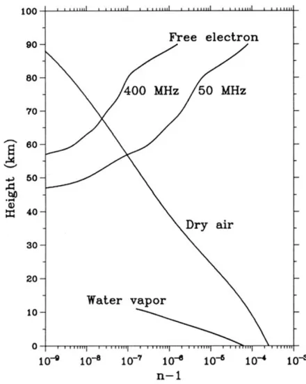
radio-wave frequency of f per second). The standard atmo-sphere model gives a height-profile ofn(Hasiguchi, 1995; Fig. 1), which decreases from ground level up to about 60 km mainly due to the second and third terms and then increases up to 100 km mainly due to the fourth term; n
is minimum at heights between 30 and 60 km. Although these values imply that the radar echo is normally barely detectable in this latter height range, Maekawaet al.(1993)
Fig. 1. Height profile of(n−1) for humidity, density (dry air) and electrons (Hasiguchi, 1995). The radio refractive index with electrons depends on radiowave frequency and illustrates two cases as 400 MHz (Arecibo Radar) and 50 MHz (Jicamarca Radar).
demonstrated that the giant Jicamarca radar can detect tur-bulence echoes by a long-time integration of the radar echo for several minutes.
The air density perturbation, which corresponds to the third term in Eq. (1) cannot be related to dynamics through an adiabatic variation of pressure since the adiabatic varia-tion is inconsistent with divV =0, which is assumed in the isotropic turbulence theory as established by Kolmogoroff, Heisenberg, Batchelor and others (Batchelor, 1953). Such an inconsistent approach for producing density perturba-tion by turbulence (Villars and Weisskopf, 1954; Tatarskii, 1971) has now been revised and a correct approach will be found.
3.
RRI Perturbation by Turbulence
Atmospheric density perturbation is, as intuitively under-stood, produced by the transport of air particles by turbu-lence velocityV along the vertical gradient in the hydro-static equilibrium atmosphere. Even with divV = 0 the density perturbation takes place, as given by the equation of continuity
∂ρ
∂t = −∇(ρV)= −Vz
dρo d z
+(second-order small terms) (2)
where Vz is the vertical (positiupward) turbulence
ve-locity component,(dρo/d z)is the hydrostatic-equilibrium
term, which is equal to(−ρo/H), withρobeing the
back-ground density, andH the scale height assumed to be
con-stant. Integration of Eq. (2) with respect to time duringτ, approximately, gives
δρt, κ2∝Vz
t, κ2τ2 (3)
whereδρ(t, κ)the perturbation of air density relative toρo
andVz(t, κ)are the Fourierκ component dependent ont;
τ is an integration time that is comparable to the turbulence correlation time; the underlining denotes the time-average. Equation (3) implies simply that the density perturbation intensity is proportional toVz2 and that the density
pertur-bation spectrum function must be the same with respect to the power spectrum of Vz2. We now resort to the
estab-lished theory of isotropic turbulence. Only isotropic tur-bulence is theoretically understood. Isotropic turtur-bulence meansVx2 = Vy2 = Vz2 whose power spectrum depends
only on wave-number magnitudeκ,E(κ), such that
E(κ)∝κ−5/3 in the inertia sub-range (4)
E(κ)∝κ−7 in the viscous sub-range. (5)
We need not enter further into turbulence theory since our concern is mainly on RRI perturbation in production and motion, not on turbulence dynamics.
The humidity perturbation of the second term in the right-hand side in Eq. (1) is transported in a similar manner as the density perturbation and the spectrum is similar to
δρ. Our understanding of the co-movement of (δρ)with turbulence is clear, with the equation of continuity in the form of following the motion (e.g. Holton, 1992), such that
Dρ
Dt = −ρdivV =0 (6)
The equation shows that the air mass moves with the flow (by turbulence and winds), maintaining the initial density, as shown in Eq. (3), irregardless of any ambient density distribution. Only in the presence of the vertically gradient distribution of the ambient density can any density pertur-bation be detected. Note that divV =0 is essential for the density-perturbation transported with turbulence plus winds (winds are divergence-free). Observations made with radars and radio-sondes are consistent with the theoretical expec-tation (Luceet al., 2001).
The mesospheric situation is different in that electron density perturbation in the fourth term in Eq. (1) takes place mainly at heights above 60 km, as shown in Fig. 1. Electro-dynamic considerations are required for turbulence trans-portation along d Ne/d z > 0 instead of dρo/d z < 0 as
only electrons are responsible for the radiowave scattering. Whilst ions co-move fairly well up to 120 km, with neu-tral particles in turbulent motion through collisions, elec-trons are strongly controlled by the geomagnetic field Bo
above 70 km since the ratio between collision frequency and gyro-frequency Ri,eis very different between ions (Ri)
and electrons (Re) in this altitude region. Ridrops to unity
at a height 120 km butRereaches this level at a much lower
height∼60 km; Ri,edecreases almost exponentially as ρo
a role in producing an electric polarization fieldEpthat
in-hibits the control of geomagnetic field. Favorably, as shown in Fig. 1, during the daytime, such a static vertical gradi-ent of Neexists above 60 km (Rastogi and Bowhill, 1976;
Lehmacheret al., 2006). Consequently, electrons can co-move with ions vertically. The details are as follows: asδρ,
δNe is produced similarly by Eqs. (2) and (3) in the
first-order magnitude as proportional toVz. Modification ofδNe
in the second order small magnitude due toV ·[grad(δNe)]
does not significantly affectδNeintensity, but does
signifi-cantly affectEp, which is modified considerably by the
sec-ond modification onδNe, as understood in electromagnetic
theory (Kato, 1965), to ultimately reach
Ep+V ×Bo=0. (7)
with
Vi=Ve=V (8)
whereVi,eare the velocity of the ions and electrons,
respec-tively, and
Vi,e=[ξi,e](Ep+V ×Bo)+V (9)
where [ξi,e] represents the mobility tensors for ions and
electrons, respectively, which are dependent on Ri,e(Kato,
1980a); Ep is produced and maintained in stationary state
with divJ =0, where J =electric current density. Even with a slight inequality betweenNeandNi, as|Ne−Ni| Ne, a largeEpis set up, following the Maxwell equation as
divEp =(Ni−Ne)e/εo (10)
in whicheis the electron charge andεothe vacuum
permit-tivity;εo=8.854·10−12farad/m. If we consider a situation
of the mesosphere and a VHF radar, |divEp| ∼ |Ep|/L,
whereL = 5 m, and(Ni−Ne) = 105/m3 = 10−3Neat z = 70 km. Using Eq. (10), we obtain Ep = 1 mV/m,
which is consistent withV =10 m/s in Eq. (7).
An additional complication is that in the presence of
Ep, Hall drifts proportional to (Ep×Bo)take place (Kato,
1980a), driving electrons and ions with different velocities and orthogonally to both Ep and Bo. However, the drifts
themselves have no divergence as div(Ep× Bo) = 0; the
drifts are also orthogonal to [grad(Ne+δNe)]. Hence, no
additional electron density perturbation occurs. We thus un-derstand that RRI perturbation(δn)in the mesosphere co-moves with turbulence eddies which, in turn, co-move with local winds. Also, the(δNe)produced suffers no loss due to
ionosphere recombination whose rate is much slower than that of turbulence correlation time as a few seconds (Kato, 1980a). Thus, we obtain another relation than that of Eq. (6) forNein the form of following the flow
D Ne
Dt = −NedivVe=0 (11)
which is based on Eq. (8); as such, the recombination loss is neglected in Eq. (11) as justified above. Further, including humidity in Eq. (1) we have
Dn
Dt =0 (12)
RRI irregularities move mainly with the winds, fluctuat-ing with turbulence. This results in the radar echo with the Doppler spectrum, whose central peak corresponds to winds, with the skirts spreading by turbulence and the in-tensity being dependent on the vertical total flow.
4.
Ob
s
ervation of Turbulence with Radar
s
In addition to tracking turbulence as wind-tracers, MST-radar observations are important tools for studying atmo-spheric turbulence dynamics.
Radars can detect echoes due to the scattering of turbu-lence, with the size of half the radar wavelength in heights lower than the critical height where 2k = κd, in whichk
denotes the radar wave-number andκd gives the minimum
scale of turbulence or the boundary between turbulence in-ertial subrange and viscous subrange (see Eqs. (4) and (5)).
κd =(ε/μ3)1/4, whereε =total power supplied from
out-side per unit time and unit mass for maintaining the turbu-lence system;μ=kinematic viscosity.κddecreases almost
exponentially with height in a manner almost proportional to air density. Thus, we can obtain the distribution of the critical height or the minimum scale of turbulence, as illus-trated in Fig. 2 (Balsley and Gage, 1980). A fairly good fitting illustrated in Fig. 2 shows that the radar observation is consistent with the isotropic turbulence theory in which
λmin ≈ 2π/κd (different from the observation showing a
factor 5.92 instead of 2π). Figure 2 contains certain er-rors about the maximum attainable height of the Jicamarca radar as 50 km, considering 50 MHz of the radar frequency or 6 m of the radar wavelength. This error should be due to
n, which is very small around 60 km as in Fig. 1, and not due to the absence of any turbulence eddies corresponding to the half wavelength of the Jicamarca radar. In actual fact, radar echoes were obtained at a height of 75 km, although
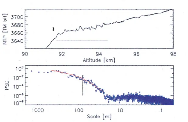
Fig. 3. Top: electron density fluctuation observed by rocket-borne Langmuir probe, September 19, 2004. The rocket launching site was on the Kwajalein Atoll, Marshall Islands. The small vertical bar indicates a fluctuation of 10%. Bottom: power spectrum of the fluctuations over heights shown by the horizontal line (top). The red line is the best fit ofE(κ)(see Eqs. (4) and (5) in text). The vertical line is located at 80±10 m, showing 9.9/κd. The minimum scale of turbulence in inertial subrange is a little longer than that in Fig. 2, givingλmin=5.92/κd.
these are not shown in Fig. 2 (Woodman and Guillen, 1974; Maekawaet al., 1993). Further, it is possible to derive a turbulence dissipation energy rateεfrom κd = (ε/μ3)1/4
whereκd is obtained from observation, as in Fig. 2, andμ
from models (Kato, 1980b);ε =0.5–1.0 W/kg at a height of 100 km.
In addition to radar observations, an important in situ ob-servation has recently been performed, obtaining a turbu-lence spectrum of the electron density (Fig. 3; Lehmacher
et al., 2006). This electron density was deduced from the electron density measurement of the Langmuir probe on-board the rockets although the electron density was also measured by incoherent scatter radar by the Altair radar at the Kwajalein Atoll and by the Faraday rotation in radio transmission between the ground and the rockets. Figure 3 gives their electron density perturbation spectrum, which is identified with E(κ) in Eqs. (4) and (5) over fairly wide range ofκ in both the inertial and viscous sub-range, both of which are bounded at about 80∓10 m in scale. Note that the boundary between the observed inertial and viscous subrange has a scale of(5.92/κd)in Fig. 2 and(9.9/κd)in
Fig. 3; as such both are different from(2π/κd), as
theo-retically expected. The observation gives anε of to 0.1– 0.3 W/kg at heights of 92–94 km, which is consistent with that obtained from Fig. 2.
5.
Conclu
s
ion
The RRI perturbation(δn)responsible for the MST radar echo is produced in the presence of static vertical gradi-ents of RRI that depend on three properties—humidity, air density and electron density. Turbulence vertical velocity transports those elements along the gradients, producing
δn, which moves with the total air flow as turbulence plus winds. Theoretically, the echo power spectrum should be the same as the vertical turbulence velocity spectrum with
κ =2k; i.e. the eddy size equals half the radar wavelength.
The co-movement takes place because of the divergence-free characteristics of turbulence and is valid even in the mesosphere, where electrons are the main component of RRI and under electromagnetic control. Based on observa-tions, the turbulenceκ-spectrum is the same as the isotropic turbulence κ-spectrum, implying that the turbulence pro-duced by gravity waves in breaking may be either isotropic or anisotropic in nature but that the turbulence spectrum is the same as that of the isotropic turbulence spectrum.
Acknowledgments. The author is grateful to Drs. T. Ogawa, D. Fritts and W. Hocking for their comments.
References
Balsley, B. B. and K. S. Gage, The MST techniques: potential for middle atmosphere studies,Pure Appl. Geophys.,118, 452–493, 1980. Batchelor, G. K.,The theory of homogeneous turbulence, pp. 46 and 114–
132, Cambridge Monograph on Mechanics and Applied Mathematics, Cambridge Univ. Press, 1953.
Hasiguchi, H., Development of an L-Band clear-air Doppler radar and its Application to planetary boundary layer observations over equatorial Indonesia, p. 10, PhD thesis, Kyoto University, January, 1995. Hocking, W. K., Measurements of turbulent energy dissipation rates in the
middle atmosphere by radar techniques, A review,Radio Sci.,20, 1403– 1422, 1985.
Holton, J. R., An introduction to dynamic meteorology (3rd edition), p. 47, Academic Press, San Diego, New York, Boston, London, Syd-ney, Tokyo, Toronto, 1992.
Kato, S., Theory of movement of irregularities in the ionosphere,Space Sci. Rev.,4, 223–235, 1965.
Kato, S.,Dynamics of the upper atmosphere, (a) pp. 141–150 (b) pp. 213– 215, Center Acad. Publ/D. Reidel Publ, Japan/Dordrecht, Boston, Lon-don, 1980.
Kato, S., Middle atmosphere research and radar observation,Proc. Jpn. Acad. Ser. B,8, 306–320, 2005.
Lehmacher, G. A., C. L. Croskey, J. D. Michell, M. Friedrich, F.-J. Lueben, M. Rapp, E. Kudeki, and D. C. Fritts, Intense turbulence observed above a mesospheric temperature inversion at equatorial latitude,Geophys. Res. Lett.,33(8), L08808, 2006.
Maekawa, Y., S. Fukao, M. Yamamoto, M. D. Yamanaka, T. Tsuda, S. Kato, and R. F. Woodman, First observation of the upper stratospheric vertical wind velocities using the Jicamarca VHF radar,Geophys. Res. Lett.,20, 2235–2238, 1993.
Rastogi, P. K. and S. A. Bowhill, Scattering of radio waves from the mesosphere-2, Evidence for intermittent mesospheric turbulence,J. At-mos. Terr. Phys.,38, 449–462, 1976.
Tatarskii, V. I.,The effect of the turbulent atmosphere on wave propaga-tion, National Technical and Information Service, pp. 74–76, Springer-field, Va, 1971.
Villars, F. and V. F. Weisskopf, The scattering of electromagnetic waves by turbulent atmospheric fluctuations,Phys. Rev.,94, 232–240, 1954. Woodman, R. F. and A. Guillen, Radar Observation of Winds and
Turbu-lence of the Stratosphere and Mesosphere,J. Atmos. Sci.,31, 493–505, 1974.