PCE-Based Approach to Worst-Case Scenario Analysis in Wireless
Telecommunication Systems
Piotr G´orniak* and Wojciech Bandurski
Abstract—In the paper, we present a novel PCE-based approach for the effective analysis of worst-case scenario in a wireless telecommunication system. Usually, in such analysis derivation of polynomial chaos expansion (PCE meta-model) of a considered EM field function for one precise set of probability densities of random variables does not provide enough information. Consequently, a number of PCE meta-models of the EM field function should be derived, each for the different joint probability density of a vector of random variables, e.g., associated with different mean (nominal) values of random variables. The general polynomial chaos (gPC) approach requires numerical calculations for each PCE meta-model derivation. In order to significantly decrease the time required to derive all of the PCE meta-models, the novel approach has been introduced. It utilizes the novel so-called primary approximation and the novel analytical formulas. They significantly decrease the number of numerical calculations required to derive all of the PCE meta-models compared with the gPC approach. In the paper, we analyze the stochastic EM fields distributions in a telecommunication system in a spatial domain. For this purpose, analysis of uncertainties associated with a propagation channel as well as with transmitting and receiving antennas was introduced. We take advantage of a ray theory in our analysis. This allows us to provide the novel method for rapid calculation of a PCE meta-model of a telecommunication system transfer function by using the separate PCE meta-models associated with antennas and a propagation channel.
1. INTRODUCTION
Simulations of electromagnetic (EM) fields cover many subjects in the area of antenna analysis and EM wave propagation prediction, e.g., [1–8]. It is often important to include the random behavior of parameters of a considered scenario in these simulations. This way, we can model, e.g., uncertainties of physical parameters of a simulated system.
One of the best-known methods of including random behavior of parameters of a given scenario in EM field simulations is the Monte Carlo method, e.g., [9, 10]. In this method, simulations are performed consecutively for variables values drawn according to an assumed probability distribution, e.g., Gaussian, Beta or uniform distributions. This method provides high accuracy in determining probability distributions of EM fields; however, it requires a lot of iterations to obtain satisfyingly accurate results. An alternative method to the Monte Carlo algorithm is the application of polynomial chaos expansion (PCE) which originates from the work of Norbert Wiener in 1938 [11] and since then was discussed in numerous articles and books, and widely used in scientific engineering, including electromagnetics, e.g., [12–17]. Our work, according to the best knowledge of the authors, is the first in which the total impact of uncertainties associated with antennas and the propagation channel on the distribution of a random electromagnetic field in a telecommunication system is analyzed. PCE enables a sufficient decrease in the computation time required to calculate the stochastic results of functions of random variables. The use of PCE for the analysis and simulation of stochastic linear systems in the
Received 20 March 2019, Accepted 8 July 2019, Scheduled 17 July 2019 * Corresponding author: Piotr G´orniak ([email protected]).
frequency-domain is based on two methods: Galerkin projection and collocation. These methods can also be used for nonlinear systems in the time-domain; however, such a case will not be considered in this work.
PCE method utilizing Galerkin projection is based on the calculation of expansion coefficients that are used to calculate statistics of considered distributions [13, 14]. The Galerkin projection has a number of convenient analytic features that make them attractive for use within analyses that extend beyond the traditional process of determining the effect of uncertainties of system physical parameters on the system response, such as local and global sensitivity analysis and design under uncertainty algorithms [18].
The collocation method requires only repetitive executions of existing deterministic solvers, so it is non-intrusive and may thus be faster [19]. However, an important issue to be kept in mind is that the aliasing errors in stochastic collocation can be significant, especially, again, for higher dimensional random spaces [19]. This indicates that the Galerkin method offers the most accurate solution of PCE coefficients of the considered function of random variables. For further comparisons of these two methods see, e.g., [12, 18, 19].
In our work, we focus on the worst-case analysis of EM field in a wireless telecommunication system for an environment whose geometrical and/or material parameters can change, for various reasons, in a random manner. This analysis is preferably carried out, as we justified above, based on the PCE method using the Galerkin projection. In this approach, the most time-consuming operation is to calculate the appropriate number of expansion coefficients in a series of orthogonal polynomials. As it is known, the number of coefficients affects the accuracy of the method, because on their basis, statistics of the stochastic process such as the average or standard deviation, etc. are calculated.
The worst-case analysis of stochastic EM field in a wireless telecommunication system requires to perform stochastic analysis repeatedly because during such analysis it is necessary to change probability density functions and/or the ranges of variation, as well as nominal values of random parameters of transmitting and receiving antennas and a propagation channel. When we have to calculate the mentioned coefficients in the PCE method repeatedly, the calculation time dramatically increases.
Our aim is to avoid this serious inconvenience by introducing the universal PCE-based approach utilizing primary approximation and the new closed-form polynomial chaos coefficients, which we call Universal Expansion Coefficients (UECs). We use the word “universal” to call our approach and our explicit analytical formulas, because in our opinion any of the nowadays intrusive or non-intrusive methods for PCE coefficients calculation can be implemented to the primary approximation which is one of the key elements of our new approach. The main idea of the proposed approach is to notice that stochastic polynomials associated with the most common probability density functions in such pairs as normal distribution — Hermite polynomials, Beta distribution — Jacobi polynomials [12, 19], etc. can be expanded in series relative to each other, and the coefficients of these expansions can be calculated by means of analytical integration resulting in known analytical relationships [20–22]. Thanks to the use of this property, we can calculate the coefficients in the PCE method only once, regardless of changes in the types of probability density function and/or variation of ranges of random parameters, what significantly shortens the simulation times in the case described above.
Let us stress that UECs have to be calculated of course but only once during the process of so-called primary approximation of the functions associated with a simulated wireless telecommunication system. In our approach, changing the values of random variables (e.g., an average and a standard deviation) or changing the range of a random variable (e.g., a random variable range for a Beta distribution) does not require, as it was already noted above, recalculation of the expansion coefficients through direct numerical integration or linear regression, which must be done for each frequency. The introduced UECs can be recalculated, as it was mentioned, using explicit analytical formulas [20–22].
The adoption of system theory approach allows the decrease of required PCE expansions order what greatly accelerates the simulation of a wireless telecommunication system.
The new results enable us to effectively analyze simulation scenarios where many (up to 10 in our simulation examples) independent random variables can be considered.
The paper is organized as follows. In Section 2, we recall the mathematical background of the PCE method and formulate the problem that is addressed in the paper. In Section 3, we present the algorithm of our UECs approach. We present the concept of the so-called primary approximation and derive polynomial chaos UECs for multiple random variables having Gaussian and Beta probability densities. We demonstrate the usefulness of system approach adoption to the considered telecommunication system. In Section 4, we use UTD ray theory and our UECs approach to mentioned worst-case analysis in a wireless telecommunication system for an exemplary scenario of diffraction of an EM wave on convex obstacles. We conclude the paper in Section 5.
2. STATEMENT OF THE PROBLEM
We recall the basic theory about PCE related to stochastic analysis. Using the general Polynomial Chaos theory (gPC) [12] we can expand the function of random variables associated with a simulated system using PCE coefficients with a polynomial basis which is orthogonal with respect to probability density (PDF) of the random variables [12]. If we assume that the transfer functionHT(ω,ξ) associated with the simulated telecommunication system depends on d independent random variables given by vector
ξ={ξ0, ξ1, ..., ξd−1}, then the expansion ofHT(ω,ξ) for pulsation sample no. scan be written as:
HT(ωs,ξ)≈
k
Ak,s d−1
n=0
ϕkn(ξn) (1)
where k={k0, k1, ..., kd−1}is a multi-index. The order of multi-indexes can be found using the Askey scheme [12], while expansion coefficients Ak,w, using the Galerkin projection [12], are:
Ak,w=
HT(ωs,ξ), d−1
n=0 ϕ(ξn)
= b0
a0 ...
bd−1
ad−1
HT(ωs,ξ) d−1
n=0 ϕ(ξn)
d−1
n=0
pn(ξn)dξd−1... dξ0
γk (2)
whereϕ(ξn) is thekn-th element of the basis of polynomials that are orthogonal for probability density functions pn(ξn) of random variables ξn in domain limits an≤ξn ≤bn, andγk=γ0·γ1·...·γd−1 is a multi-normalization factor [12], whilekn is then-th element of multi-index k. It should be noticed that for Gaussian distribution numerical integration of Eq. (2) can be in practice truncated and consequently performed within finite limits, e.g.,μ−5σ, μ+ 5σ, hereμandσare the mean and standard deviation of a Gaussian PDF. Using the expansion coefficients in Eq. (2) the mean and standard deviation of random transfer function HT(ω,ξ) for pulsation samplesωs can be found as follows [12]:
μw = A{0,0,...,0},w (3)
σw =
k={0,0,...,0}
γk2·Ak,w (4)
We address in the paper the problem of worst-case analysis in the wireless telecommunication system. The transfer function of a telecommunication system with random parameters can be written as follows:
HT(ω,ξ) = R
r=1
HCrATFsω,ξrATFs ·HCrCTFω,ξrCTF (5)
whereHCATFs
r (ω,ξrATFs) is the joint transfer function of transmitting and receiving antennas associated with the r-th ray path which originates at the point of EM field source and ends at the observation point; HCCTF
random variables of antennas transfer functions corresponding to r-th ray path, while ξrCTF is the vector of random variables of transfer function of the r-th ray. It is possible that transfer functions
HCCTF
r (ω,ξCTFr ) depend on the same vector of random variables, e.g., when rays interact with the same obstacles or it is assumed that parameters of obstacles are deterministic, while antenna positions are random variables.
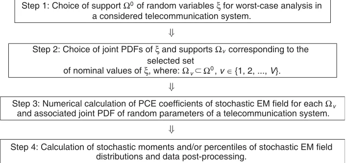
In order to define the problem of worst-case analysis in a telecommunication system, we define support Ω0 of random variables ξ for which the worst-case analysis need to be made. This support can be associated, e.g., with limits of spatial coordinates of antennas positions. Then support Ω0 is sampled into much smaller supports, e.g., supports Ωv,v∈ {1,2, ..., V} which correspond to a selected set of nominal values of ξ. Supports Ωv need to reflect uncertainties which can be met in a real life, e.g., uncertainty in determining the position of antennas. We assume that each of supports Ωv can be associated with Gaussian, Beta or Uniform PDF. After support Ω0, supports Ωv and associated PDFs are chosen, we perform simulations of considered telecommunication system repeatedly. In the gPC approach, we need to perform a numerical calculation of PCE coefficients for every execution of the simulation. The diagram showing this approach can be presented as follows.
3. THE UEC APPROACH
3.1. The Diagram of the UEC Approach
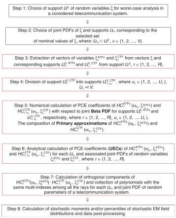
When the worst-case analysis in a telecommunication system is performed according to the algorithm shown in Fig. 1, the calculation time can be not acceptable, because it grows fast, as the simulations of stochastic EM field propagation are repeated. It is the consequence of repeated numerical calculations of PCE coefficients for every support Ωv. We present now the diagram of our UEC approach which ensures substantial reduction of computation times of worst-case analysis in a telecommunication system. The novel blocks in the diagram are indicated by red frames. The diagram can be presented as in Fig. 2.
Step 1: Choice of support Ω of random variables ξ for worst-case analysis in a considered telecommunication system.
0
Step 2: Choice of joint PDFs of ξ and supports Ω corresponding to the selected set
of nominal values of ξ, where: Ω ⊃ Ω , v ∈ {1, 2, ..., V}. v
v 0
Step 3: Numerical calculation of PCE coefficients of stochastic EM field for each Ω and associated joint PDF of random parameters of a telecommunication system. v
Step 4: Calculation of stochastic moments and/or percentiles of stochastic EM field distributions and data post-processing.
Figure 1. The diagram of the gPC approach for worst-case analysis in a telecommunication system.
The first two steps of the UEC approach are the same as in the gPC approach. In the first step of the novel part of the UEC approach, we assign an appropriate subset of variablesξ to antennas transfer function as it is indicated in (5). The complementary subset of variables is assigned to transfer functions of rays. It should be noted that vectors ξrATFsand ξrCTFdo not overlap. We also decompose support of variables ξ into supports Ω0,ATFsr and Ω0,CTFr for variables ξATFsr and ξCTFr , respectively.
In the next step, we divide support Ω0,CTFr into Ur supports Ω0,CTFr,ur for the transfer function of
Step 1: Choice of support Ω of random variables ξ for worst-case analysis in a considered telecommunication system.
0
Step 2: Choice of joint PDFs of ξ and supports Ω corresponding to the selected set
of nominal values of ξ, where: Ω ⊃ Ω , v ∈ {1, 2, ..., V}. v
v 0
Step 8: Calculation of stochastic moments and/or percentiles of stochastic EM field distributions and data post-processing.
Step 3: Extraction of vectors of variables ξ and ξ from vectors ξ and corresponding supports Ω and Ω from support Ω , r ∈ {1, 2, ..., R}.
r ATFs r CTF r 0, ATFs r
0, CTF 0
Step 4: Division of support Ω into supports Ω , where u ∈ {1, 2, ..., U }, U Vr > > .
r 0, CTF
r, u 0, CTF
r r r
Step 5: Numerical calculation of PCE coefficients of HC (ω , ξ ) and HC (ω , ξ ) with respect to joint Beta PDF forsupports Ω and
Ω , respectively, where r ∈ {1, 2, ..., R}, u ∈ {1, 2, ..., U }. The composition of Primary approximations of HC (ω , ξ ) and
HC (ω , ξ ).
r ATFs r ATFs s CTF
r, ur s r CTF
r 0, ATFs
r, u 0, CTF
r r r
rATFs s
s r ATFs r CTF r CTF
Step 6: Analytical calculation of PCE coefficients (UECs) of HC (ω , ξ ) and HC (ω , ξ ) for each Ω and associated joint PDFs of random variables
ξ and ξ , where r ∈ {1, 2, ..., R}. r ATFs
s rATFs CTF
r, ur s r CTF v r ATFs r CTF
Step 7: Calculation of orthogonal components of
HC (ω , ξ ) .HC (ω , ξ ) and collection of polynomials with the same multi-indexes among all the rays for each Ω and joint PDF of random
paremeters of a telecommunication system. r
ATFs
s ATFsr rCTF s rCTF
v
Figure 2. The diagram of the UEC approach for worst-case analysis in a wireless telecommunication system.
particular, we need to divide the portion of support Ω0,CTFr,ur which corresponds to spatial coordinates.
The results of numerical experiments, which was performed by us for 2 spatial dimensions, indicate that a good choice for the spatial area included in Ω0,CTFr,ur is 4−16λ
2, whereλis a wavelength. It is not required
to divide the support Ω0,ATFsr because it does not include spatial coordinates, therefore dynamics of variation of HCrATFs(ω,ξrATFs) is much lower than for the case of transfer function HCrCTF(ω,ξCTFr ). We used the Matlab-based package called UQLab [24] to perform the mentioned numerical experiments. When primary approximations of HCrATFs(ωs,ξATFsr ) and HCrCTF(ωs,ξCTFr ) are derived we can apply them to explicit analytical formulas, called UECs, which are the PCE coefficients of
HCATFs
r (ωs,ξrATFs) andHCrCTF(ωs,ξrCTF) for supports Ωv and selected joint PDFs of ξATFsr and ξrCTF. The final step of the novel part of the UEC approach is the derivation of PCE of each transfer function associated with the path of ray no. r, as well as the collection of polynomials with the same multi-indexes in order to obtain the PCE of a telecommunication system transfer function.
3.2. The Primary Approximation
In order to derive the universal expansion coefficients (UECs), we present the primary approximation which was introduced in the previous subsection.
The primary approximation of an exemplary transfer function HC(ω,ξ) for pulsation sample ωs by analogy to Eq. (1) is as follows:
HC(ωs,ξ)≈
q
Cq,w d−1
n=0 Pα0β0
qn (f1(ξn)) (6)
whereqn is then-th element of multi-index q,
f1(ξn) =ξn 2
bn−an −
bn+an
bn−an, f1(an) =−1, f1(bn) = 1 (7)
and Pqαn0β0(ξn) is a Jacobi polynomial of the qn−th order with shape parameters α0 and β0, whilean
andbnare the lower and higher limits of primary approximation for variableξn. It should be noted that the number of coefficients Cq,w in Eq. (6) is a finite and minimal number that satisfies the accepted approximation error criterion. We chose this polynomial basis, as we obtained the best approximation results in our experiments using Jacobi polynomials, especially for transfer functions whose specified domains are limited. Coefficients Cq,w can be calculated using Galerkin projection as follows:
Cq,w= 1 γk
HC(ωs,{f2(ξ0), ..., f2(ξd−1)}), d−1
n=0 Pα0β0
qn (ξn)
= 1
γk 1
−1 ...
1
−1
HC(ωs,{f2(ξ0), ..., f2(ξd−1)}) d−1
n=0 Pα0β0
qn (ξn)
d−1
n=0
pBetan (α0, β0, ξn)dξd−1... dξ0 (8)
where
f2(ξn) = ξn
bn−an
2 +
bn+an
2 , f2(−1) =an, f2(1) =bn (9)
pBetan (α, β, ξ) = 2(α+β+1) Γ(α+β+ 2)
Γ(α+ 1)Γ(β+ 1)(1−ξ)
α(1 +ξ)β (10)
However, other methods for calculation of PCE coefficients can be used. We use UQLab [24] for numerical calculation of Cq,w. Among several options of PCE coefficients calculation in UQLab, we choose orthogonal matching pursuit (OMP) which is connected with Sobol indices calculation.
The necessary but time-consuming numerical calculations required to obtain coefficients Cq,w are performed for freely chosen parameters α0 and β0 and only once for a given HC(ωs,ξ). We use α0 =β0≤1 for the best primary approximation results.
3.3. The Universal Expansion Coefficients
CoefficientsCq,w from the previous subsection are tabulated and used to derive our universal expansion coefficients (UECs). We limit our consideration to the case of random variableξnthat can have Gaussian or Beta distribution. Beta distribution enables modeling a symmetric and asymmetric PDF, as well as the uniform PDF. Let new arbitrary parameters of Gaussian probability density function ofξnare mean μn and standard deviation σn. The appropriate parameters of Beta distribution are shape parameters αn and βn while their new ranges are cn ≤ ξn ≤ dn [12]. Then UECs, denoted by Uk,w, are the polynomial chaos expansion coefficients of HC(ωs,ξ) with respect to chosen probability distributions of random variables ξ. The expansion formula with UECs takes the form:
HC(ωs,ξ)≈
k
Uk,w d−1
n=0
whereϕkn(ξn) can be a Hermite or Jacobi polynomial for Gaussian or Beta distribution, respectively [12]. Functionf2(ξn) for Gaussian distribution is:
f3G(ξn) = ξn−μn σn
(12)
while for Beta distribution, by analogy to Eq. (7), we have:
f3B(ξn) =ξn 2
dn−cn −
dn+cn
dn−cn f3(cn) =−1 f3(dn) = 1 (13) It should be noted that the number of multi-indexes kis not higher than the number of multi-indexes
q because the range of possible values of ξn in Eq. (11) must be a subset of the range of ξn for which the primary approximation in Eq. (6) was derived. The range of possible values of ξn for the case of Beta distribution is cn ≤ ξn ≤ dn but also for the case of a Gaussian distribution this range can in practice be limited toμn−M·σn≤ξn≤μn+M·σn. We useM = 5 (the UECs are valid for such an assumption). When we take advantage of the primary approximation in Eq. (6) and use the Galerkin projection, the initial formula for our UECs takes the form:
Uk,w≈ 1 γk
q
Cq,w d−1
n=0 Pα0β0
qn (f1(f4(ξn))),
d−1
n=0
ϕkn(ξn)
(14)
Functionf4(ξn) for Gaussian distribution is:
f4G(ξn) =σn·ξn+μn (15)
while for Beta distribution, by analogy to Eq. (9), we have:
f4B(ξn) =ξndn−cn
2 +
dn+cn
2 , f4(−1) =cn, f4(1) =dn (16)
Then we transform a Jacobi polynomial of theqn-th order in Eq. (14) into a sum of Hermite polynomials of maximum order qn-th [25]. After the transformation, Eq. (14) takes the following form:
Uk,w≈ 1 γk
q
Dq,w d−1
n=0
Hqn(f1(f4(ξn))),
d−1
n=0
ϕkn(ξn)
(17)
whereHl(x) is a Hermite polynomial of orderl and:
Dq,w =D{q0, q1, ..., qd−1}, w=
i0≥q0, i1≥q1, ..., id−1≥qd−1
C{i0, i1, ..., id−1}, w d−1
n=0 Bin
qn (18)
whereBin
qn is the weight of Jacobi polynomial of orderin-th that compose a Hermite polynomial of order
qn-th and can be calculated as in [21].
The UEC in Eq. (17) can be given in the following form:
Uk,w≈ 1 γk
q
Dq,w d−1
n=0
Skn,qn(ξn) (19)
When ξn has Gaussian distribution, then factorSkn, qn(ξn) takes the form:
SkGn, qn(ξn) = +∞
−∞
Hqn(f1(f
G
4 (ξn)))Hkn(ξn)
e−ξ
2
n
2
√
2πdξn (20)
while for Beta distribution we have:
SkBn, qn(ξn) = 1
−1
Hqn(f1(f
B
After simplifying Eqs. (20) and (21), factor Skn, qn(ξn) for Gaussian distribution takes the following
form:
SkGn, qn(ξn) = +∞
−∞ Hqn(z
Gauss
D (ξn))Hkn(ξn)
e−ξ
2
n
2
√
2πdξn (22)
where
zDGauss(ξn) = gGaussn ·ξn+hGaussn (23)
gGaussn = 2σn bn−an
(24)
hGaussn = 2μn−bn−an
bn−an (25)
while for Beta distribution we have:
SkBn, qn(ξn) = 1
−1 Hqn(z
Beta
D (ξn))Pkαnn, βn(ξn)pBetan (αn, βn, ξn)dξn (26)
where
zBetaD (ξn) = gnBeta·ξn+hBetan (27)
gnBeta = dn−cn bn−an
(28)
hBetan = dn+cn−bn−an bn−an
(29)
The Hermite polynomial of the sum of arguments has the following property [26]:
Hl(x+y) = l j=0 l j
xl−jHj(y) (30)
We apply the above property to Eq. (22) with substitutions x = hGaussn , y = gGaussn ·ξn, as well as to Eq. (26) with substitutions x = gBeta
n ·ξn, y = hBetan . When we apply the results of integrals of
the forms ∞
−∞Hl1(z)Hl2(z) exp(−0.5z
2)dz and 1 −1
zpHl1(z)Plα,β2 (1−z)α(1 +z)βdz, as well as subsequent
transformations, we derive the closed form formulas forSkn, qn(ξn). Forξnwith Gaussian PDF, we have:
SkGn, qn(ξn) =
hGauss n
1−(gGauss n )−2
kn · kn j=0
(gGauss
n )2−1
(hGauss
n )2
j
Q(j, qn, kn) (31)
where Q(j, qn, kn) does not depend on μn or σn, therefore, they can be tabulated as follows. When (j−kn) = 0,2,4,6..., we have [21]:
Q(j, qn, kn) = qn!
(qn−j)!
j−kn
2
!(√2)j−kn
(32)
while Eq. (32) is 0 for the remaining values of (j−kn). The corresponding formula to Eq. (31) for the case of Beta PDF is:
SkBn,qn(ξn) = qn j=0 qn j Hj
hBetan gBetan qn−jIn (33)
whereInis 0 for qn−j < kn, and for qn−j =kn it can be calculated by:
In=Ikn = Γ(kn+αn+ 1)Γ(kn+βn+ 1) Γ(2kn+αn+βn+ 2) 2
while for the rest of the cases:
In=Ikn
qn−j kn
F21(kn−qn+j, αn+kn+ 1, αn+βn+ 2kn+ 2,2) (35)
whereF21(., ., ., .) is a Gaussian hypergeometric function [27].
One can see that SkGn,qn(ξn) in Eq. (20) and SkBn,qn(ξn) in Eq. (21) can be calculated without any integration but using explicit formulas (31) and (33), respectively. As a consequence, UECs Uk,s in Eq. (19) can also be calculated this way for each function HCrATFs(ωs,ξrATFs) and HCrCTF(ωs,ξrCTF) what is performed in step 6 of our UEC approach shown in Fig. 2. In the final novel part of our UEC approach, shown in Fig. 2, we calculate PCE coefficients of HT(ωs,ξ) and perform elementary operations with orthogonal polynomials what is presented in the next subsection.
3.4. The PCE of a Telecommunication System Transfer Function
We take advantage of the fact that the transfer function of the telecommunication system is a sum of transfer functions associated with rays which originate in the point of EM field source and reach an observation point. Each of these transfer functions is the product of antennas transfer function associated with ray no. rand a transfer function of ray no.r, which are called by us,HCrATFs(ω,ξATFsr ) and HCrCTF(ω,ξCTFr ), respectively. The transfer function associated with the ray no. r for pulsation sample ωs is defined as follows.
HCr(ωs,ξr) =HCrATFs
ωs,ξATFsr ·HCrCTFωs,ξrCTF (36)
The method that we use to derive PCE coefficients of Eq. (36) is analogous to methods used in literature for calculation of PCE coefficients for dynamic systems, e.g., [23]. Let us assume thatξATFsr ={ξ0, ξ1},
ξCTF
r = {ξ2, ξ3}, and ξr = {ξ0, ξ1, ξ2, ξ3}, while the expansions of the functions HCrATFs(ωs,ξrATFs), HCrCTF(ωs,ξCTFr ) are as follows:
HCrATFs(ωs, ξ0, ξ1) ≈
j
AHr,ATFsj ·ΨATFsr,j (ξ0, ξ1) (37)
HCrCTF(ωs, ξ2, ξ3) ≈
k
AHr,CTFk ·ΨCTFr,k (ξ2, ξ3) (38)
The goal is to expand function HCr(ωs, ξ0, ξ1, ξ2, ξ3) into the following form:
HCr(ωs, ξ0, ξ1, ξ2, ξ3)≈
m
AHr,m·Ψr,m(ξ0, ξ1, ξ2, ξ3) (39)
where: j, k, m are multi-indexes, Ψr,m(ξ0, ξ1, ξ2, ξ3) = ϕr,m0(ξ0) ·ϕr,m1(ξ1)·ϕr,m2(ξ2) ·ϕr,m3(ξ3), Ψr,j(ξ0, ξ1) = ϕr,j0(ξ0) ·ϕr,j1(ξ1), Ψr,k(ξ2, ξ3) = ϕr,k0(ξ2)·ϕr,k1(ξ3). When we substitute expansion in Eqs. (39), (37), (38) into Eq. (36), we obtain:
m
AHr,m·Ψr,m(ξ0, ξ1, ξ2, ξ3) =
j
AHr,ATFsj ·ΨATFsr,j (ξ0, ξ1)·
k
AHr,CTFk ·ΨCTFr,k (ξ2, ξ3) (40)
In order to derive PCE coefficient of HCr(ωs, ξ0, ξ1, ξ2, ξ3) with multi-index m, we apply Galerkin projection to both sides of Eq. (40) using polynomial Ψr,m(ξ0, ξ1, ξ2, ξ3) and associated joint PDF. When we take advantage of orthogonal property [12] of the polynomials, we obtain:
AHr,m =
j
Hqm,j·AHr,ATFsj (41)
where:
Hqm,j =
k
AHr,CTFk αm(j,k,m) (42)
αm(j,k,m) = 1 γr,m
ΨATFsr,j (ξ0, ξ1),Ψr,CTFk (ξ2, ξ3),Ψr,m(ξ0, ξ1, ξ2, ξ3)
In the case when functions ΨATFsr,j (ξ0, ξ1), ΨCTFr,k (ξ2, ξ3), Ψr,m(ξ0, ξ1, ξ2, ξ3) belong to the same orthogonal bases, expression (43) can be easily calculated by the formula:
αm(j,k,m) =
1, if {m0, m1}={j0, j1} ∧ {m2, m3}={k0, k1}
0, otherwise. (44)
When the lengths of multi-indexes j,k and m equal dATFs,dCTF and d=dATFs+dCTF, respectively, the above formula can be generalized as follows:
αm(j,k,m) =
1, if∀(0≤n≤dATFs−1)(jn=mn)∧ ∀(0≤n≤dCTF−1)(kn =mn+dATFs)
0, otherwise. (45)
When polynomial chaos expansions of HCrATFs(ωs,ξrATFs) and HCrCTF(ωs,ξrCTF) include PATFs and PCTF components, respectively, polynomial chaos expansion ofHCr(ωs,ξr) includesPATFs·PCTF components. The vector of multi-index m of each product in the left side of Eq. (40) is created by concatenation of vectors of multi-indexes j and k belonging to factors which are included in this product.
When polynomial chaos expansion of Eq. (36) for each ray in a wireless telecommunication system is known, we derive polynomial chaos expansion of Eq. (5). It is assumed by us that all random variables associated with antennas are independent. Let us assume that two rays lead from the point of source of EM field to the observation point. Then we have vectors of random variables ξATFs1 , ξ2ATFs, ξ1CTF,
ξCTF
2 on the right side of Eq. (5). Let us assume also in the first illustrative example thatξ1ATFs={ξ0},
ξATFs
2 ={ξ1, ξ2},ξ1CTF={ξ3},ξCTF2 ={ξ3, ξ4}. Consequently, transfer functionHT(ω,ξ) depends on the vector of random variablesξ={ξ0, ξ1, ξ2, ξ3, ξ4}, while its PCE for pulsation sampleωscan be given as follows:
HT(ωs,ξ)≈
m1
AH1,p1·Ψ1,p1(ξ0, ξ3) +
m2
AH2,p2 ·Ψ2,p2(ξ1, ξ2, ξ3, ξ4) (46)
where multi-indexes p1 and p2, using the notation as in Eqs. (39), (44), (45), are {m10,0,0, m11,0} and {0, m20, m21, m22, m23}, respectively. All of the components of expansion (46) belong to the same orthogonal basis and have unique multi-indexes. It should be noted thatϕ0(ξ) = 1 for each orthogonal basis in gPC theory. Consequently, polynomials Ψ1,p1(ξ) depend only on variables ξ0 and ξ3, while polynomials Ψ2,p2(ξ) depend on variables ξ1, ξ1, ξ3 and ξ4. In the second illustrative example, we assume that ξ1ATFs = {ξ0, ξ1}, ξ2ATFs = {ξ2, ξ3}, ξCTF1 = {ξ4, ξ5}, ξ2CTF = {ξ4, ξ5}. Consequently, the vector of random variables of transfer functionHT(ω,ξ) is ξ ={ξ0, ξ1, ξ2, ξ3, ξ4, ξ5}. Then by analogy to expansion (46), we could write:
HT(ωs,ξ)≈
m1
AH1,p1 ·Ψ1,p1(ξ0, ξ1, ξ4, ξ5) +
m2
AH2,p2·Ψ2,p2(ξ2, ξ3, ξ4, ξ5) (47)
where multi-indexes p1 = {m10, m11,0,0, m12, m13}, p2 = {0,0, m20, m21, m22, m23}; however, expansion (47) includes components which have the same multi-indexes. The not unique multi-indexes are formed by m10 = 0, m11 = 0, m20 = 0, m21 = 0, m12 = m22, m13 = m23. Consequently, the components of expansion (47) which have the same multi-indexes have to be added all together in order to derive polynomial chaos expansion of HT(ω,ξ).
Having in mind the two presented illustrative examples the following conclusion can be made. When two or more ray transfer functions HCrCTF(ω,ξrCTF) depend on the same vector of random variables then components of PCEs of HCrATFs(ωs,ξrATFs)·HCrCTF(ωs,ξrCTF), which have the same multi-indexes, need to be collected in order to derive PCE of HT(ωs,ξ). Then the analogous rule to this, which is given below Eq. (47), should be applied. In other cases, all components of PCEs of HCrATFs(ωs,ξrATFs)·HCrCTF(ωs,ξrCTF) become the components of PCE of HT(ωs,ξ).
4. NUMERICAL EXAMPLES
slope diffraction defined in the frequency-domain [28, 29] and a corresponding creeping ray trajectory in the scenario. Only the rays which give the major contribution to the overall field at the observation point of receiving antenna PR are taken into account. The antenna position is established at pointPT. The aim of the simulation is to analyze the worst-case scenario of EM wave propagation in the presence of exemplary convex objects. This would concern a scenario when the transmitting antenna and the receiving antenna are shadowed by convex objects. The diffraction takes place on a cascade of three cylinders, see Fig. 3. The objects are assumed to be perfect conductors. The radius of each convex object is 0.75 m. We assume that the centers of the objects lie in one line. The distance between the centers of each consecutive pair of objects equals 2 m.
Figure 3. The scenario of a creeping wave propagating along three convex obstacles modeled by circular cylinders. The position of a transmitting antenna is represented by random variables ξx-x dimension, ξy-y dimension.
Transmitting antenna radiates EM wave whose frequency is 6 GHz. The point of a transmitting antenna PT may change its position within the red line with a step of 2 cm (36 positions). The line is 5 m away from the center of convex object No. 1.
of 15 positions of transmitting antenna is defined as follows.
HT(ω,ξ) = 2
r=1
HCrATFs
ξT, M agr , ξrT, P h, ξrR, M ag, ξrR, P h
·HCrCTF(ω, ξx, ξy) (48)
where
HCrATFs
ξrT, M ag, ξrT, P h, ξR, M agr , ξR, P hr
=ξrT, M ag·e−j·ξrT, P h·ξR, M ag
r ·e−j·ξ
R, P h
r (49)
and HCCTF
r (ω, ξx, ξy) is the transfer function of ray no. r which is calculated using the uniform theory of diffraction [28]. The slope of the diffracted field is calculated as in [29]. We assume that an EM wave is TE-polarized. As we mentioned earlier we assume a two-dimensional case of EM wave propagation.
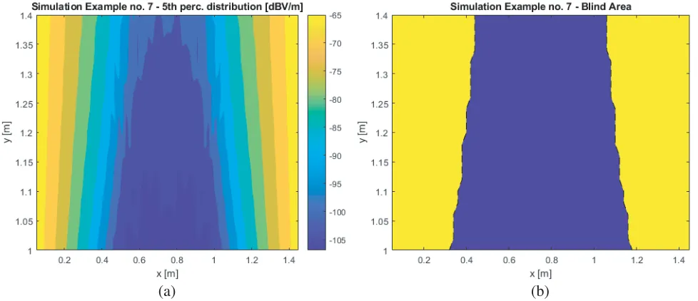
We analyze the worst-case scenario of an electric field amplitude for each 0.02 m×0.02 m square at the receiving antenna site. We organize our calculations as follows. We assume that from the environmental protection perspective, for an electric field amplitude, the incident electric field cannot be larger than 0 dBV/m (1 V/m). We calculate the local minimum of an electric field amplitude for all nominal positions of the receiving antenna (300 positions). We calculate the local minimum value as thenth percentile of the calculated stochastic electric field amplitude. We repeat this procedure for all positions of the transmitting antenna. Then out of all local minima at each nominal position of the receiving antenna, we choose the minimal value, which is called the global minimum. If the global minimum for a given position of the receiving antenna is not lower than some threshold value associated with, e.g., receiver sensitivity, then the transmission between transmitting and reviving antennas will be successful for (100−n)% of cases. Otherwise, this connection can be broken. We consider 5-th percentile of an electric field amplitude to calculate global minima. We will assume in the next subsections that the exemplary threshold value of electric field amplitude at the receiving site is−85 dBV/m. The area for which the value of the global minimum of an electric field amplitude is below the threshold value is called the “Blind area”.
We present 7 simulation examples in the paper for 7 different ranges of uncertainties of antennas transfer functions. We will present the changes of the “Blind area” between the chosen simulation examples and the corresponding distribution of values of global minima for the observation area shown in Fig. 3. We show also the results of the relative error between UEC results and the Monte Carlo results for the chosen simulation examples. We do not show the error between UEC results and the gPC results; however, we note that this error is very small and that its maximum value is not bigger than 0.5% for all simulation examples. However, we do present the comparison of the times necessary to run the simulations using the Monte Carlo method, gPC approach and our UEC approach for all simulation examples in a tabular form.
As we mentioned in Section 3.2, we take advantage of the freeware Matlab-based package called UQLab [24] to obtain the results of the primary approximation for the UEC approach, as well as for numerical calculations of PCE coefficients in the gPC approach. We choose the orthogonal matching pursuit (OMP) method with Sobol indices calculation to calculate PCE coefficients in UQLab.
The values of parameters of PDFs assumed for the mentioned simulation examples are shown in Table 1. The lower and higher limits of supports of uniform random variables which model uncertainties of antennas transfer functions are denoted in Table 1 bycandd, respectively. The first column in Table 1 refers to the number of simulation example. The next 4 columns in Table 1 contain the pairs ofc and dvalues. The first pair corresponds to the magnitude of antennas transfer functions, while the second to the phase of antennas transfer functions.
Table 1. The values of parameters of PDFs assumed for the simulation examples.
Sim. Ex. No.
ATFs Magn. Uncertainty
ATFs Phase Uncertainty
c
V/m V/m
d
V/m V/m
c[◦] d[◦]
1 1 1 0 0
2 0.90 1.10 −10 10
3 0.85 1.15 −20 20
4 0.80 1.20 −30 30
5 0.75 1.25 −40 40
6 0.70 1.30 −50 50
7 0.65 1.35 −60 60
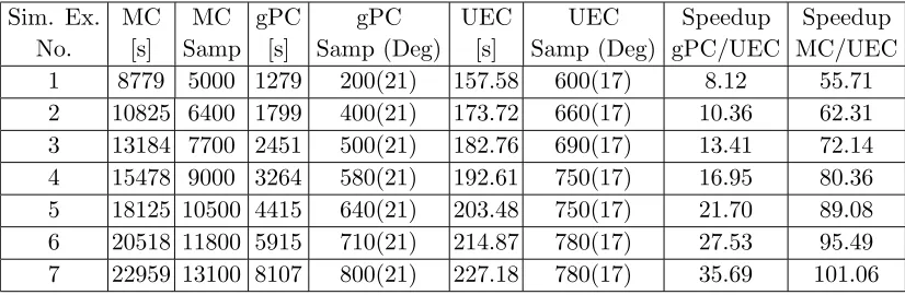
Table 2. Parameters and times associated with calculations of the simulation examples.
Sim. Ex. No.
MC [s]
MC Samp
gPC [s]
gPC Samp (Deg)
UEC [s]
UEC Samp (Deg)
Speedup gPC/UEC
Speedup MC/UEC
1 8779 5000 1279 200(21) 157.58 600(17) 8.12 55.71
2 10825 6400 1799 400(21) 173.72 660(17) 10.36 62.31 3 13184 7700 2451 500(21) 182.76 690(17) 13.41 72.14 4 15478 9000 3264 580(21) 192.61 750(17) 16.95 80.36 5 18125 10500 4415 640(21) 203.48 750(17) 21.70 89.08 6 20518 11800 5915 710(21) 214.87 780(17) 27.53 95.49 7 22959 13100 8107 800(21) 227.18 780(17) 35.69 101.06
approach is presented in the last two columns of Table 2. The size of spatial support for the primary approximation of each ray transfer function is 0.1 m×0.1 m.
As it is shown by the results included in Table 2, our UEC approach provides a substantial saving of simulation time for the case of worst-case analysis in a stochastic telecommunication system when compared to the gPC approach and especially to the Monte Carlo method. In our exemplary scenario, which is shown in Fig. 3, we considered 36 positions of a transmitting antenna and 300 nominal positions of a receiving antenna. As a consequence, we performed 10800 simulations of propagation of stochastic EM wave for the scenario shown in Fig. 3. The time reduction provided by our UEC approach is the larger the bigger is the number of simulations which are required to perform the worst-case analysis of a considered telecommunication system.
It is important to note that we use the gPC approach according to the diagram shown in Fig. 1. This approach implements the non-intrusive method for calculations of PCE coefficients. We could modify this approach by adding the steps analogous to the steps with numbers 3, 4, 6 and 7 of the UEC approach. Then the speedup of our UEC approach compared to this modified gPC approach is 4.63 for the case of deterministic antennas transfer functions (simulation example No. 1) and is similar for the case of the other 6 simulation examples. This speedup is obtained when the size of spatial support for the modified gPC approach is 0.02 m×0.02 m. This speedup is about 50% lower when the size of spatial support for primary approximation of each ray transfer function is 0.05 m×0.05 m. The times of calculations associated with the primary approximations of rays transfer functions are by far the biggest part of the whole simulation time. It is caused by high dynamics of each ray transfer function variation in the spatial domain.
(a) (b)
Figure 4. (a) The distribution of global minima obtained by using the UEC approach presented in the decibel scale and (b) the “Blind area” for simulation example No. 1.
(a) (b)
Figure 5. (a) The distribution of global minima obtained by using the UEC approach presented in the decibel scale and (b) the “Blind area” for simulation example No. 7.
corresponding “Blind area” for simulation examples No. 1 and No. 7 are shown in Fig. 4 and Fig. 5, respectively.
(a) (b)
Figure 6. The relative error of UEC global minima results (a) for simulation example No. 1 and (b) for simulation example No. 7.
(a) (b)
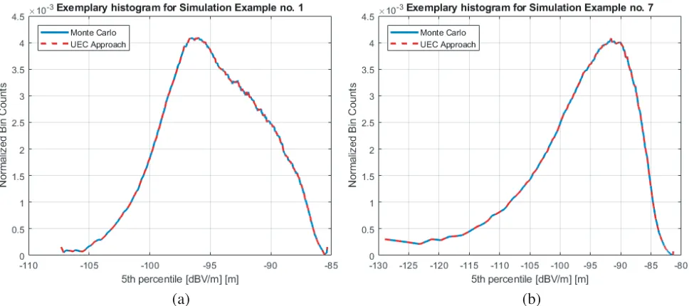
Figure 7. The smoothed histograms of an electric field amplitude at nominal observation point x = 1.26 m, y = 0.75 m calculated by using the MC method and the UEC approach for simulation examples (a) No. 1 and (b) No. 7.
operations [24]. It is achieved without deterioration of the accuracy of obtained PCE meta-models, and thus the accuracy of the distributions of a random amplitude of an electric field compared with the gPC and Monte Carlo approaches. We observed similar results of speedup and accuracy of analysis of random electric field for other simulation examples in which geometrical optics (GO) and UTD were used. However, they are not included in the paper because of the space limitation.
5. CONCLUSIONS
We presented in the paper a new PCE-based UEC approach to the fast and accurate simulation of worst-case scenario in a wireless telecommunication system. In this case, multiple simulations should be performed, each with a different set of PDFs of random variables. Namely, we presented in Section 3.3 new, closed-form analytical formulas which enable fast calculation of coefficients of polynomial chaos expansion. It is done in step 6 of our UEC approach. These formulas rely on primary approximations introduced in Section 3.2. The numerical calculation of primary approximation coefficients in Eq. (6) has to be performed once for each support introduced in Step 4 of the UEC approach. This process is by far the most time-consuming step in the UEC approach. In step 7 of the UEC approach, we proposed the novel intrusive method for calculation of PCE expansion of a stochastic EM field in a wireless telecommunication system. Our UEC approach requires the description of the transmission in the telecommunications system, i.e., its transfer function in the frequency domain which depends on random parameters (described using independent random variables). The approach relies on the nature of ray tracing simulation and on separating antennas transfer function and the ray transfer function for each ray. The analytical UECs, presented in Section 3.3, are dedicated to Gaussian and Beta distributions. These two probability densities cover a very wide range of probability densities considered in the literature for simulations of stochastic EM field distributions. It should be noted that uniform probability density can be modeled by Beta distribution as in the simulation examples presented in Section 4. The limitation of the UEC approach is related to the frequency of the EM field which needs to be expanded by using PCE. We observed that at about 30 GHz and higher frequencies the OMP, as well as the other non-intrusive methods of PCE coefficients calculation are hardly efficient. In order to obtain a sufficient quality primary approximation, very high order approximations need to be used. Consequently, simulation times dramatically increase. It is the common limitation of the gPC and UEC approaches. We are currently working on the application of our approach to the full-wave analysis (e.g., FDTD method, method of moment). It turns out that the application of the approach presented in this paper, using the so-called “primary approximations” and analytical formulas presented in this article, also gives a significant speedup of PCE meta-models calculation. The first results regarding the FDTD method are promising; however, they require further work and possible results will be published later.
ACKNOWLEDGMENT
The work was supported by the Ministry of Science and Higher Education.
REFERENCES
1. Alibakhshi-Kenari, M., M. Naser-Moghadasi, R. A. Sadeghzadeh, B. S. Virdee, and E. Limiti, “Traveling-wave antenna based on metamaterial transmission line structure for use in multiple wireless communication applications,”AEUE Elsevier — International Journal of Electronics and
Communications, Vol. 70, No. 12, 1645–1650, 2016.
2. Alibakhshi-Kenari, M., M. Naser-Moghadasi, R. A. Sadeghzadeh, B. S. Virdee, and E. Limiti, “A new planar broadband antenna based on meandered line loops for portable wireless communication devices,” Radio Science, Vol. 51, No. 7, 1109–1117, 2016.
4. Alibakhshi-Kenari, M., M. Naser-Moghadasi, R. A. Sadeghzadeh, B. S. Virdee, and E. Limiti, “New compact antenna based on simplified CRLH-TL for UWB wireless communication systems,”
International Journal of RF and Microwave Computer-Aided Engineering, Vol. 26, No. 3, 217–225,
2016.
5. Alibakhshi-Kenari, M., M. Naser-Moghadasi, R. A. Sadeghzadeh, B. S. Virdee, and E. Limiti, “Dual-band RFID tag antenna based on the hilbert-curve fractal for HF and UHF applications,”
IET Circuits, Devices and Systems, Vol. 10, No. 2, 140–146, 2016.
6. Schafer, T. M. and W. Wiesbeck, “Simulation of radiowave propagation in hospitals based on FDTD and ray-optical methods,”IEEE Trans. on Antennas and Propagation, Vol. 53, No. 8, 2381–2388, 2005.
7. Hosseini Tabatabaei, S. A., M. Fleury, N. N. Qadri, and M. Ghanbari, “Improving propagation modeling in urban environments for vehicular ad hoc networks,” IEEE Trans. on Intelligent
Transportation Systems, Vol. 12, No. 3, 769–783, 2011.
8. Lertsirisopon, N., G. S. Ching, M. Ghoraishi, J.-I. Takada, I. Ida, and Y. Oishi, “Investigation of non-specular scattering by comparing directional channel characteristics from microcell measurement and simulation,”IET Microwaves, Antennas and Propagation, Vol. 2, No. 8, 913–921, 2008.
9. Ozgun, O. and M. Kuzuoglu, “Monte Carlo-based characteristic basis finite-element method (MCCBFEM) for numerical analysis of scattering from objects on/above rough sea surfaces,”IEEE
Trans. on Geoscience and Remote Sensing, Vol. 50, No. 3, 769–783, 2012.
10. Wagner, R. L., J. Song, and W. C. Chew, “Monte Carlo simulation of electromagnetic scattering from two-dimensional random rough surfaces,”IEEE Trans. on Antennas and Propagation, Vol. 45, No. 2, 235–245, 1997.
11. Wiener, N., “The homogeneous chaos,”American Journal of Mathematics, Vol. 60, No. 4, 897–936, 1938.
12. Xiu, D., Numerical Methods for Stochastic Computation. A Spectral Method Approach, Princton University Press, New Jersey, 2010.
13. Edwards, R. S., A. C. Marvin, and S. J. Porter, “Uncertainty analyses in the finite-difference time-domain method,” IEEE Trans. Electromagn. Compat., Vol. 52, No. 1, 155–163, 2010.
14. Kersaudy, P., S. Mostarshedi, S. Sudret, and O. Picon, “Stochastic analysis of scattered field by building facades using polynomial chaos,” IEEE Trans. on Antennas and Propagation, Vol. 62, No. 12, 6382–6393, 2014.
15. Boeykens, F., H. Rogieri, and L. Vallozzi, “An efficient technique based on polynomial chaos to model the uncertainty in the resonance frequency of textile antennas due to bending,”IEEE Trans.
on Antennas and Propagation, Vol. 62, No. 3, 1253–1260, 2014.
16. Larbi, M., I. S. Stievano, F. Canavero, and P. Besnier, “Identification of main factors of uncertainty in a microstrip line network,” Progress In Electromagnetics Research, Vol. 162, 61–72, 2018. 17. Haarscher, A., P. De Doncker, and D. Lautru, “Uncertainty propagation and sensitivity analysis
in ray-tracing simulations,” Progress In Electromagnetics Research M, Vol. 21, 149–161, 2011. 18. Eldred, M. S., “Design under uncertainty employing stochastic expansion methods,”International
Journal for Uncertainty Quantification, Vol. 1, No. 2, 119–146, 2011.
19. Xiu, D., “Fast numerical methods for stochastic computations: A review,” Commun. Comput.
Phys., Vol. 5, Nos. 2–4, 242–272, 2009.
20. G´orniak, P. and W. Bandurski, “A new approach to polynomial chaos expansion for stochastic analysis of EM wave propagation in an UWB channel,” Wireless Days, Toulouse, March 23–25, 2016.
21. G´orniak, P. and W. Bandurski, “Universal approach to polynomial chaos expansion for stochastic analysis of EM field propagation on convex obstacles in an UWB channel,” 12th European
Conference on Antennas and Propagation, EuCAP 2016, Davos, April 10–14, 2016.
Propagation, EuCAP 2017, Paris, March 20–24, 2017.
23. Spina, D., D. Dhaene, and L. Knockaert, “Polynomial chaos-based macromodeling of general linear multiport systems for time-domain analysis,” IEEE Trans. Microwave Theory and Techniques, Vol. 65, No. 5, 1422–1433, 2017.
24. Marelli, S. and B. Sudret, “UQLab user manual — Polynomial chaos expansions,”Report
UQLab-V1.0-104, Chair of Risk, Safety and Uncertainty Quantification, ETH Zurich, 2017.
25. Bella, T. and J. Reis, “The spectral connection matrix for any change of basis within the classical real orthogonal polynomials,”Mathematics 2015, Vol. 3, No. 2, 382–397, 2015.
26. Weisstein, E. W., CRC Concise Encyclopedia of Mathematics, CRC Press, London, 2003.
27. Forrey, R. C. and J. Reis, “Computing the hypergeometric function,” Journal of Computational
Physics, Vol. 137, No. 1, 79–100, 1997.
28. McNamara, D. A.,Introduction to the Uniform Geometrical Theory of Diffraction, Artech House, Boston, 1990.
29. Koutitas, G. and C. Tzaras, “A UTD solution for multiple rounded surfaces,” IEEE Trans. on