Efficient Alignment Algorithms for DNA Sequencing Data

(1)

Scholarship@Western

Electronic Thesis and Dissertation Repository

1-31-2018 11:00 AM

Efficient Alignment Algorithms for DNA Sequencing Data

Nilesh Vinod Khiste

The University of Western Ontario

Supervisor Lucian Ilie

The University of Western Ontario NA

The University of Western Ontario Graduate Program in Computer Science

A thesis submitted in partial fulfillment of the requirements for the degree in Doctor of Philosophy

Follow this and additional works at: https://ir.lib.uwo.ca/etd

Part of the Bioinformatics Commons, Computational Biology Commons, Genomics Commons, and the Other Computer Engineering Commons

Recommended Citation Recommended Citation

Khiste, Nilesh Vinod, "Efficient Alignment Algorithms for DNA Sequencing Data" (2018). Electronic Thesis and Dissertation Repository. 5192.

https://ir.lib.uwo.ca/etd/5192

This Dissertation/Thesis is brought to you for free and open access by Scholarship@Western. It has been accepted for inclusion in Electronic Thesis and Dissertation Repository by an authorized administrator of

(2)

The DNA Next Generation Sequencing (NGS) technologies produce data at a low cost,

en-abling their application to many ambitious fields such as cancer research, disease control,

per-sonalized medicine etc. However, even after a decade of research, the modern aligners and

assemblers are far from providing efficient and error free genome alignments and assemblies

respectively. This is due to the inherent nature of the genome alignment and assembly

prob-lem, which involves many complexities. Many algorithms to address this problem have been

proposed over the years, but there still is a huge scope for improvement in this research space.

Many new genome alignment algorithms are proposed over time and one of the key diff

er-entiators among these algorithms is the efficiency of the genome alignment process. I present a

new algorithm for efficiently finding Maximal Exact Matches (ME M s) between two genomes:

E-MEM (Efficient computation of maximal exact matches for very large genomes).

Comput-ing MEMs is one of the most time consumComput-ing step durComput-ing the alignment process. E-MEM can

be used to find MEMs which are used as seeds in a genome aligner to increase its efficiency.

The E-MEM program is the most efficient algorithm as of today for computing MEMs, and it

surpasses all competitors by large margins.

There are many genome assembly algorithms available for use, but none produces perfect

genome assemblies. It is important that assemblies produced by these algorithms are evaluated

accurately and efficiently.This is necessary to make the right choice of the genome assembler

to be used for all the downstream research and analysis. A fast genome assembly

evalua-tor is a key facevalua-tor when a new genome assembler is developed, to quickly evaluate the

out-come of the algorithm. I present a fast and efficient genome assembly evaluator called LASER

(Large genome ASsembly EvaluatoR), which is based on a leading genome assembly evaluator

QUAST, but significantly more efficient both in terms of memory and run time.

The NGS technologies limit the potential of genome assembly algorithms because of short

read lengths and nonuniform coverage. Recently, third generation sequencing technologies

have been proposed which promise very long reads and a uniform coverage. However, this

(3)

indels. The long read sequencing data are useful only after error correction obtained using self

read alignment (or read overlapping) techniques. I propose a new self read alignment algorithm

for Pacific Biosciences sequencing data: HISEA (Hierarchical SEed Aligner), which has very

high sensitivity and precision as compared to other state-of-the-art aligners. HISEA is also

integrated into Canu assembly pipeline. Canu+HISEA produces better assemblies than Canu

with its default aligner MHAP, at a much lower coverage.

Keywords: Bioinformatics, De novo genome assembly, E-MEM, Genome assembly

eval-uation, HISEA, HiSeq, Illumina, LASER, Long read alignment, Maximal exact matches,

Next-generation sequencing, Pacific Biosciences, Sequence alignment

(4)

However, it was a very tough decision to leave behind a set career path. I could not have done

it without the support of my family. I dedicate this work to them.

(5)

I would like to express my sincere gratitude to everyone involved in the completion of

this dissertation. Most importantly, I would like to thank my supervisor Dr. Lucian Ilie for

introducing me to the amazing research field of Bioinformatics and string algorithms. His

con-tinuous encouragement helped me to explore various interesting problems in Bioinformatics

and use my research to propose efficient solutions for some of them. I really appreciate his

extraordinary patience in reviewing my manuscripts, research proposals, presentations and this

dissertation. His critical feedback and suggestions were always helpful in enhancing the

qual-ity of these documents. I am very grateful to my supervisor for the valuable time he spent

discussing my ideas and guiding me.

I am thankful to the Department of Computer Science at the University of Western Ontario

for awarding me with the Western Graduate Research Scholarship (WGRS). I am also grateful

to the Ministry of Training, Colleges and Universities (Ontario) for awarding me the Ontario

Graduate Scholarship (OGS) for two consecutive years.

I am also thankful to my examiners and members of my supervisory committee Dr. Ming

Li, Dr. Kathleen Hill, Dr. Roberto Solis-Oba, Dr. Anwar Haque and Dr. Kaizhong Zhang. I

am thankful to my colleagues Dr. Mike Molnar and Yiwei Li for all the technical discussions

around various topics. I would like to thank my friends and family members for their constant

support and encouragement which kept me going and led to the completion of this research

work, which is one of the biggest accomplishments of my life.

(6)

Abstract i

Dedication iii

Acknowlegements iv

List of Figures x

List of Tables xiii

List of Appendices xv

1 Introduction 1

1.1 DNA sequencing . . . 3

1.1.1 Sanger method . . . 3

1.1.2 Next generation sequencing . . . 5

1.1.3 Third generation sequencing . . . 7

1.2 Maximal Exact Matches . . . 10

1.3 Assembly Evaluation . . . 11

1.4 Sequence Alignment . . . 12

2 Maximal Exact Matches: E-MEM 14 2.1 Background . . . 14

2.1.1 Basic Notions and Definitions . . . 14

Suffix tree and suffix array . . . 15

(7)

LCP interval . . . 17

2.1.2 MUMmer . . . 17

2.1.3 Vmatch . . . 17

Computation of MEMs using Enhanced Suffix Array . . . 20

2.1.4 SparseMEM . . . 21

Computation of MEMs using Sparse Suffix Array . . . 22

Parallelization technique in sparseMEM . . . 23

2.1.5 EssaMEM . . . 24

2.1.6 BackwardMEM . . . 25

Computing Parent Intervals . . . 26

Computation of MEMs using the FM-index . . . 27

Compressed Suffix Array implementation . . . 28

2.1.7 SlaMEM . . . 29

Sampled LCP Array . . . 29

Sampled Smaller Values . . . 29

2.1.8 Comparison . . . 30

2.2 E-MEM algorithm . . . 31

2.3 Sequence Storage . . . 34

2.4 Efficientk-mer Storage . . . 34

2.5 Hash Table and hashing function . . . 35

2.6 Searching query . . . 36

2.7 Handling redundant MEM matches . . . 37

2.8 Dealing with ambiguous bases (N) . . . 38

2.9 Split parameter - memory reduction . . . 39

2.10 Very large number of MEMs . . . 39

2.11 Output formats . . . 40

(8)

2.12.1 Evaluation . . . 41

2.12.2 Human vs Mouse . . . 42

Minimum MEM length 100 . . . 42

2.12.3 Human vs Chimp . . . 47

2.12.4 Triticum aestivum vs Triticum durum . . . 51

2.13 Conclusions . . . 54

3 Assembly Evaluation: LASER 55 3.1 Background . . . 55

3.2 QUAST Introduction . . . 57

3.2.1 Contig sizes . . . 58

3.2.2 Misassemblies and structural variations . . . 59

3.2.3 Genome representation . . . 59

3.2.4 NAx and NGAx . . . 60

3.2.5 Visualizations . . . 60

Cumulative length . . . 61

Nx plot . . . 61

NAx plot . . . 62

NGx plot . . . 62

NGAx plot . . . 63

GC content plot . . . 63

3.3 LASER Improvements . . . 64

(9)

3.3.2 Code remodeling . . . 65

3.3.3 NUCmer changes . . . 65

3.4 Results . . . 65

4 Genome Alignment: HISEA 69 4.1 Background . . . 69

4.1.1 BLASR . . . 73

4.1.2 DALIGNER . . . 74

4.1.3 GraphMap . . . 74

4.1.4 MHAP . . . 75

4.1.5 Minimap . . . 77

4.2 HISEA Introduction . . . 77

4.3 HISEA algorithm . . . 78

4.3.1 Storing reads and hashing the reference set . . . 78

4.3.2 Searching the query set . . . 79

4.3.3 Filtering and clustering . . . 80

4.3.4 Computing and extending alignments . . . 83

4.4 Alignment evaluation method . . . 86

4.4.1 Compute Dynamic Programming Alignment . . . 87

4.4.2 Sensitivity computation . . . 88

4.4.3 Specificity computation . . . 89

4.4.4 Precision computation . . . 90

4.4.5 F1score computation . . . 91

4.5 Results . . . 91

4.5.1 Alignment results . . . 92

Standalone comparison . . . 92

(10)

Sensitivity vs overlap size . . . 97

MHAP sketch size and Minimap minimizers . . . 98

4.5.2 Assembly results . . . 100

Sensitivity of HISEA and MHAP - assembly pipeline . . . 101

5 Conclusions and Future Research 116 5.1 Conclusions . . . 116

5.2 Future research . . . 117

Bibliography 119 A E-MEM Results For MEM Computation 126 A.1 Human vs Mouse . . . 127

A.1.1 Minimum MEM length 100 . . . 127

A.2 Human vs Chimp . . . 129

A.3 Triticum aestivum vs Triticum durum . . . 131

Curriculum Vitae 132

(11)

1.1 DNA molecule structure [7] . . . 2

1.2 Comparison of Sanger methods - gel-electrophoresis ladder (left) and flores-cent labels (right) [53]. The arrow shows the direction of DNA sequence from 5’ end to 3’ end. . . 5

1.3 Bridge amplification of DNA fragments in Illumina technologies [41]. . . 7

1.4 (A) ZMW containing template and polymerase. (B) Event sequence of DNA incorporation [20]. . . 8

1.5 Pacific Biosciences unbiased coverage [9]. . . 9

1.6 Pacific Biosciences Consensus Accuracy [8] . . . 9

1.7 Alignment example. . . 12

2.1 The suffix tree forS =acaaacatat[2]. . . 15

2.2 The lcp-interval tree of the stringS =acaaacatat[2]. . . 18

2.3 k-mer hashing technique: only thek-mers shown are stored . . . 34

2.4 Efficient k-mer matching . . . 36

2.5 Redundant MEMs . . . 37

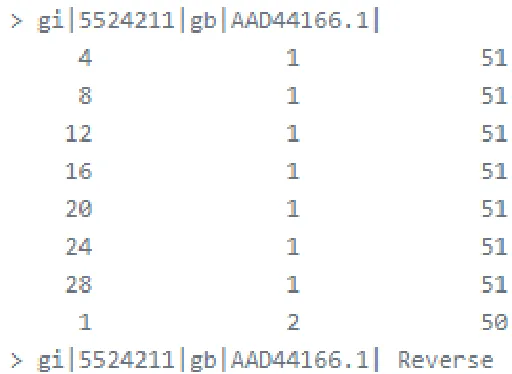
2.6 Example: 3-column output . . . 40

2.7 Example: 4-column output . . . 41

2.8 Homo sapiensvsMus musculus; MEMs of minimum length 100. The top plot is for serial mode, the bottom for parallel. Note the different scale of the plots. . 44

2.9 Homo sapiensvsMus musculus; MEMs of minimum length 300. The top plot is for serial mode, the bottom for parallel. Note the different scale of the plots. . 46

(12)

is for serial mode, the bottom for parallel. Note the different scale of the plots. . 48

2.11 Homo sapiensvsPan troglodytes; MEMs of minimum length 300. The top plot is for serial mode, the bottom for parallel. Note the different scale of the plots. . 50

2.12 Triticum aestivumvsTriticum durum; MEMs of minimum length 100. . . 52

2.13 Triticum aestivumvsTriticum durum; MEMs of minimum length 300. . . 53

3.1 N50 example. . . 56

3.2 QUAST genome assembly evaluation flow [24]. . . 56

3.3 Structural Variations [25] . . . 59

3.4 Cumulative contig length . . . 61

3.5 Nxvalues . . . 61

3.6 NAxvalues . . . 62

3.7 NGxvalues . . . 62

3.8 NGAxvalues . . . 63

3.9 GCcontent . . . 64

3.10 Visual performance comparison of QUAST and LASER . . . 67

4.1 Alignment example. . . 69

4.2 Global vs Local Alignment [14] . . . 70

4.3 Overview of BLASR algorithm; Chaissonet al.[16] . . . 73

4.4 MinHash overview; Berlinet al.[6] . . . 76

4.5 Allk-mer matches between readsqandrbefore (a) and after (b) clustering. . . 80

4.6 Computing the alignment. The dark grey region contains all k-mer matches and is extended by the light grey ones usingk0-mer matches. . . 83

4.7 Relationship between alignments reported by program and real alignments . . . 86

4.8 Sensitivity as a function of mean overlap length. . . 97

4.9 Mummer plot forE.coli30x . . . 105

(13)

4.11 Mummer plot forS.cerevisiae30x . . . 107

4.12 Mummer plot forS.cerevisiae50x . . . 108

4.13 Mummer plot forC.elegans30x . . . 109

4.14 Mummer plot forC.elegans50x . . . 110

4.15 Mummer plot forA.thaliana30x . . . 111

4.16 Mummer plot forA.thaliana50x . . . 112

4.17 Mummer plot forD.melanogaster30x . . . 113

4.18 Mummer plot forD.melanogaster50x . . . 114

(14)

1.1 Output information for Illumina large scale sequencing platforms. . . 6

2.1 FM-index of the stringS =acaaacatat . . . 16

2.2 Count arrayC[p] . . . 17

2.3 Suffix array of the stringS = acaaacatatwith LCP: Longest Common Prefix, BWT: BurrowsWheeler transform, SA: Suffix Array, ISA: Inverse Suffix Array, child table and suffix link tables. . . 20

2.4 Sparse suffix array of the stringS = acaaacatatwith LCP, and ISA . . . 21

2.5 PS V andNS Vtables of the stringS = acaaacatat. . . 27

2.6 A nutshell comparison of applications. Notations used in the table: ST (Suf-fix Tree); ESA (Enhanced Suffix Array); SSA (Sparse Suffix Array); ESSA (Enhanced Sparse Suffix Array); LCP (Longest Common Prefix); CT (Child Table); BS (Binary Search). . . 31

2.7 Genomes used for testing . . . 42

3.1 Sequencing data used for comparison . . . 66

3.2 Assembly generation and evaluation time comparison . . . 66

3.3 QUAST and LASER comparison . . . 67

4.1 Smith-Waterman alignment for sequences TGGTTACT and TAGTAGTTACT . 72 4.2 SMRT datasets used in for evaluation . . . 92

4.3 Comparison for the 1 Gbp datasets. . . 93

4.4 Time and memory comparison for the 1 Gbp datasets. . . 95

(15)

4.6 Effect of increasing sketch size on MHAP sensitivity. . . 99

4.7 Effect of increasing number of minimizers on Minimap sensitivity. . . 100

4.8 Sensitivity, specificity, precision andF1-score for HISEA and MHAP program output within the Canu pipeline. . . 101

4.9 Assembly comparison; Canu assembler is used with MHAP and HISEA as read aligners. . . 103

4.10 Assembly time and space comparison. . . 104

A.1 Homo sapiensvsMus musculus; MEMs of minimum length 100. . . 127

A.2 Homo sapiensvsMus musculus; MEMs of minimum length 300. . . 128

A.3 Homo sapiensvsPan troglodytes; MEMs of minimum length 100. . . 129

A.4 Homo sapiensvsPan troglodytes; MEMs of minimum length 300. . . 130

A.5 Triticum aestivumvsTriticum durum; MEMs of minimum length 100. . . 131

A.6 Triticum aestivumvsTriticum durum; MEMs of minimum length 300. . . 131

(16)

Appendix A . . . 126

(17)

Introduction

It has been known for decades that evolution is a change in inherited characteristics of

biolog-ical populations. In 1859, Charles Darwin was the first person to propose a scientific theory

of evolution which was associated with the population genetics theory. Population genetics is

the study of the frequency and interactions ofallelesandgenesin populations. A gene is the molecular unit of heredity of a living organism. The genetic information within a particular

gene may not be the same for different organisms and therefore different copies of a gene may

give different instructions. Each unique form of a single gene is called anallele. As an exam-ple, one allele for the gene for hair color could instruct the body to produce a lot of pigment,

producing black hair, while a different allele of the same gene might give garbled instructions

that fail to produce any pigment, giving white hair.

Genes are made from a long molecule called DNA (Deoxyribonucleic acid), which is

copied and inherited across generations. DNA is a molecule that encodes the genetic

instruc-tions used in the development and functioning of all known living organisms and many viruses.

DNA molecules consist of a double stranded structure forming a double helix. The two DNA

strands are known as polynucleotides since they are composed of simpler units called

nu-cleotides. Each nucleotide is composed of a nitrogen-containing nucleobase, either guanine

(G), adenine (A), thymine (T), or cytosine (C) as well as a monosaccharide sugar called

(18)

oxyribose and a phosphate group. The nucleotides are joined to one another in a chain by

covalent bonds between the sugar of one nucleotide and the phosphate of the next, resulting

in an alternating sugar-phosphate backbone. According to base pairing rules (A with T and C

with G), hydrogen bonds bind the nitrogenous bases of the two separate polynucleotide strands

to make double-stranded DNA. The two strands of DNA run in opposite directions. The two

ends of a single stranded DNA in forward direction are identified by 5’ (five prime) and 3’

(three prime) ends. Figure 1.1 shows a DNA molecule structure with A-T and G-C hydrogen

bonds.

Figure 1.1: DNA molecule structure [7]

DNA sequencing is the process of determining the precise order of nucleotides within a

DNA molecule. It includes any method that is used to determine the order of the four bases

in a strand of DNA. The advent of rapid DNA sequencing methods has greatly accelerated

(19)

1.1 DNA sequencing

The attempt for gene sequencing started in the early 1970s and the first known successful gene

sequencing was done by Gilbert and Maxam [23] in 1973. They were able to produce a gene

sequence of 24 base pairs by a method known as wandering-spot analysis. The method was

very labor intensive and time consuming when used with real biological datasets, given the

ex-treme length of biological sequences. This situation changed when Frederick Sanger developed

several faster, more efficient techniques to sequence DNA. Frederick Sanger’s work [51] in this

area was groundbreaking and it led to his being a recipient of the Nobel Prize in Chemistry in

1980. Although the basic Sanger method was still being used to sequence whole genomes, time

and cost considerations continued to make it expensive, thus limiting the number of genomes

that could be completed. Using Sanger sequencing, the Human Genome Project took more

than 10 years and incurred a cost of nearly $3 billion [1].

1.1.1 Sanger method

The Sanger sequencing method [51], also know as chain-termination method requires a

single-stranded DNA template, a DNA primer, a DNA polymerase, normal

deoxynucleotidetriphos-phates (dNTPs), and modified di-deoxynucleotidetriphosdeoxynucleotidetriphos-phates (ddNTPs) for sequencing to be

performed. In this method, the templates are divided into four separate sequencing reactions

containing DNA polymerase and all four dNTPs. Only one ddNTP is added to each sample

which produces many DNA polymerized sequences of varying length each ending in

corre-sponding ddNTP. These polymerized sequences can then be separated by a technique called

gel-electrophoresisbased on sequence length. The base identification is performed by dena-turing polyacrylamide-urea gel with each of the four reactions. The terminal ddNTP indicates

whether an A, T, G, or C occurs in that position on the template strand. When a gel is stained

with a DNA-binding dye, the DNA fragments can be seen as bands, each representing a group

(20)

light.

Over the years, this process has been greatly simplified. The sequencing can be performed

in a single reaction. The chain termination based kits are commercially available which are

ready to use and contain all the reagents needed for sequencing. The DNA polymerized

se-quences are terminated by incorporating fluorescently labeled nucleotide thereby producing a

DNA ladder which makes it easier to determine the DNA sequence of the original DNA

frag-ment. The process is repeated many times until it is guaranteed that a ddNTP is incorporated

at every single position of template DNA. At this point, the samples contain fragments of

dif-ferent lengths, ending at each of the nucleotide positions in the DNA template. Figure 1.2

shows a comparison between two sequencing techniques - a gel based radioactive method and

a fluorescent method. The image on the left is an example of the Sanger method using the

gel-electrophoresis ladder. The image on the right is the automated Sanger method using

flo-rescent labels through a capillary tube [53]. The short fragments move faster and pass through

the capillary tube first followed by longer fragments. The smallest fragment is created by

in-corporating only one nucleotide after the primer. The color of the dye is used for detection of

nucleotide at the end of the tube, which produces original DNA sequence - one nucleotide at a

time.

The Sanger method was expensive and time consuming due to usage of gels. It limited

the application of this method to small viruses and bacterial genomes. New sequencing

meth-ods [54] utilizing automated reloading of the capillaries with polymer matrix instead of slab

gels were introduced to speed up the sequencing process. The automated sequencing methods

increased total throughput and decreased costs gradually for Sanger sequencing. These

auto-mated methods were successfully employed in the human genome project and reduced both

cost and time required to complete the project.

Sanger sequencing provided remarkable opportunities to life sciences and improved the

knowledge and understanding of cellular mechanisms and diseases. However, limitations

(21)

Figure 1.2: Comparison of Sanger methods - gel-electrophoresis ladder (left) and florescent labels (right) [53]. The arrow shows the direction of DNA sequence from 5’ end to 3’ end.

application to various genomics projects. Several new methods for DNA sequencing were

de-veloped in the mid to late 1990s. These techniques comprise manynext-generation sequencing (NGS) methods. All of NGS techniques achieve high throughput by simultaneously

sequenc-ing many DNA sequence templates.

1.1.2 Next generation sequencing

NGS techniques are inexpensive and produce an enormous amount of sequencing data in a

short amount of time. The data produced by NGS is much cheaper and faster to obtain than the

Sanger reads, however the data contain more errors. Some of the NGS platforms are Roche 454,

Ion Torrent and Illumina. The most popular NGS platform is Illumina, which has dominated

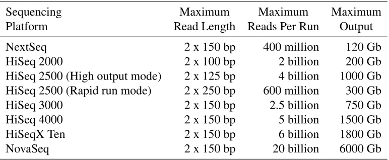
sequencing space for the last decade. It can sequence small fragments of DNA, calledreads, that are between 100 to 300 bp long. The details of current Illumina platforms are listed in

(22)

Table 1.1: Output information for Illumina large scale sequencing platforms.

Sequencing Maximum Maximum Maximum

Platform Read Length Reads Per Run Output

NextSeq 2 x 150 bp 400 million 120 Gb HiSeq 2000 2 x 100 bp 2 billion 200 Gb HiSeq 2500 (High output mode) 2 x 125 bp 4 billion 1000 Gb HiSeq 2500 (Rapid run mode) 2 x 250 bp 600 million 300 Gb HiSeq 3000 2 x 150 bp 2.5 billion 750 Gb HiSeq 4000 2 x 150 bp 5 billion 1500 Gb HiSeqX Ten 2 x 150 bp 6 billion 1800 Gb NovaSeq 2 x 150 bp 20 billion 6000 Gb

The Illumina sequencing technology can be summarized in three core steps - amplify,

se-quence and analyze. The process begins by breaking up a DNA sese-quence into smaller

frag-ments. These fragments are attached with adapters. An adapter is the oligos bound to the 5’

and 3’ end of each DNA fragment which act as a reference points throughout the rest of the

process. The modified DNA is immobilized on a flow cell surface, calledcluster station, which facilitates access to enzymes while ensuring stability of surface bound DNA templates. The

DNA is then amplified by adding unlabeled nucleotides through a process called bridge am-plification. During this process, the enzymes incorporate nucleotides to build double-stranded bridges on the surface and then make copies of it. Several million copies of double stranded

DNA are generated in each cluster of the flow cell. Primers and flourescently labeled

termina-tors are added to the flow cell that allow primers to add only one nucleotide at a time. A camera

is used to take a picture of the cell and a computer determines the base by the wavelength of

the fluorescent tag. The process of Illumina sequencing is described in Figure 1.3.

One of the biggest drawback of Illumina technology is the short read length produced by it.

Illumina sequencing platform also suffers from biases. Abiasin DNA sequencing technology is defined as the deviation from the ideal uniform distribution of reads. Both, the short reads

and bias limit the application of Illumina sequencing data in downstream applications.

(23)

Figure 1.3: Bridge amplification of DNA fragments in Illumina technologies [41].

technologies. One of the most promising third generation sequencing technology is Pacific

Biosciences SMRT(Single Molecule, Real Time)sequencing. The SMRT sequencing technol-ogy produces very long reads (> 60Kbp) and uniform coverage across the genome but has

error rates even higher than NGS technologies.

1.1.3 Third generation sequencing

SMRT relies on sequencing by synthesis approach and real time detection of incorporated

flu-orescently labeled nucleotides. It is a parallelized single molecule DNA sequencing method.

The two core elements of SMRT sequencing are zero-mode waveguides (ZMWs) and phos-pholinked nucleotides. The process begins by affixing a single DNA molecule and DNA poly-merase at the bottom of the ZMW as shown in Figure 1.4 (A). ZMWs allow light to illuminate

only at the bottom of the well as a DNA molecule is incorporated. Phospholinked nucleotides

allow observation of the DNA strand as it is produced. The four bases are tagged with diff

er-ent florescer-ent dyes and are attached to the phosphate chain of the nucleotide. When the DNA

(24)

detec-tor detects the fluorescent signal and the base call is made according to the color of the dye.

Figure1.4 (B), shows the details of the incorporation process.

Figure 1.4: (A) ZMW containing template and polymerase. (B) Event sequence of DNA in-corporation [20].

The Pacific Biosciences SMRT technology offers long reads with relatively higher error

rate (15−20%) compared to NGS technologies. The technology is free from biases due to

GC rich regions of the genome [49]. For NGS, the coverage levels drop significantly in GC

rich regions which makes it impossible to reconstruct these regions of the genome. Since these

biases do not exist in SMRT technology, it ensures the uniform coverage of entire genome.

Coverageis defined as the average number of times each base pair in a genome is sequenced. Given a dataset ofnreads of lengthlwith a genome length of L, the coverage is defined as:

Coverage= n_L×l

Unlike NGS, the single molecule technology does not require DNA amplification and

there-fore sampling related biases are also not present. A coverage plot against GC% was plotted for

A.thalianagenome and shown in Figure 1.5.

The sampling of reads and the errors in reads are completely random. Hence, with sufficient

coverage, the effect of high error rate can be mitigated. Figure 1.6 shows a plot between phred

quality value and amount of coverage. Phred quality value (QV) is defined asQ=−10 log10P, where P is the base calling error probabilities. Clearly, it can be seen that as the coverage

(25)

Figure 1.5: Pacific Biosciences unbiased coverage [9].

consensus. A consensussequence is a DNA sequence which is used to describe a number of related but non identical sequences. Aperfect consensussequencing data has 100% coverage of nucleotides in reference genome.

(26)

1.2 Maximal Exact Matches

In the remaining part of the introduction, we describe the problems that we are interested in

this thesis. In this section, we describe the Maximal Exact Matches (MEMs) computation

prob-lem followed by two other sections where we describe the assembly evaluation and sequence

alignment problems. MEMs play an important role in genome alignments and comparisons

when sequences are relatively similar. MEMs act as seeds in the alignment of high-throughput

sequencing reads and are used as anchor points in genome-genome comparisons. Recently,

MEMs have been used in Jabba [42] for error correction of long reads obtained from third

gen-eration sequencing platforms like Pacific Biosciences and Oxford Nanopore. MEMs are exact

matches between two sequences that cannot be extended in either direction without allowing

for a mismatch. A related concept with an additional constraint of having a single unique copy

in each sequence, called maximal unique matches (MUMs), is also used widely for the same

purpose. There are two popular algorithmic approaches have been used in past for

computa-tion of MEMs. In the first approach, a compressed index structure of concatenacomputa-tion of both

sequences is created and MEMs are computed by iterating over the index structure. This

ap-proach has higher memory requirement as both the sequences are used for index creation. In

the second approach, the index is created for one of the sequences (reference), and MEMs are

computed by matching the second sequence (query) against the index. The second approach

has obvious advantages over the first approach in terms of size and re-usability of the index

structure.

The E-MEM [30] algorithm is based on the second approach discussed above, where it

cre-ates an index for the reference sequence and then computes MEMs by matching and extending

k-mers from the query sequence. Ak-mer is defined as a small sequence ofkcharacters in the DNA sequence. E-MEM surpasses the state-of-the-art in MEM computation. The details of

(27)

1.3 Assembly Evaluation

Genome assembly is one of the most fundamental problems in Bioinformatics, with many

applications. Agenome assembler is a program which is used to construct the original DNA (or genome) sequence from the reads produced by DNA sequencing. The degree of accuracy

in recreating the original DNA from fragments (reads) depends on the error rate, coverage

and the relationship between the length of reads and the length of repeats in the DNA being

assembled. Assuming low error rate and sufficient coverage, the solution largely depends on

the lengths of reads and repeats. A repeat is a pattern of DNA sequences which occur in multiple copies throughout the genome. If all repeats are shorter than read length, the solution

is trivial. If some repeats are larger than read length, the solution requires trying an exponential

number of arrangements which can be computationally very expensive. If most of the repeats

are larger than read length, it might be impossible to reconstruct the genome even after trying

an exponential number of arrangements. The coverage plays an equally important role, no

coverage or very low coverage can adversely affect the accuracy and reconstruction of the

genome. Based on the available sequencing technologies, most of the full genome sequences

cannot be reconstructed efficiently and reliably. Rather, a fragmented and generally error-prone

assembly is produced. Numerous algorithms have been developed and newer algorithms are

proposed all the time, trying to achieve accurate genome assembly and longer contigs. A contig

is a set of overlapping DNA segments that together represent a consensus region of DNA. It is

important to evaluate the quality of produced assembly before being used in further research.

The LASER [29] program is a highly efficient version of the QUAST [25] program, which

is more than five times faster and requires only half the memory for large genomes. LASER

replaces MUMmer [34, 19, 18] with E-MEM for the MEM computation module in QUAST

and makes other changes which result in significant performance improvements. The details

(28)

1.4 Sequence Alignment

Genome or sequence alignment algorithms have been around for more than half a century now.

These algorithms have been improved over the years to enhance performance. Figure 1.7 shows

a simple example of genome alignment between sequences GAACTA and TAGAA. The gaps

or mismatches in the alignment are shown with an underscore character.

Figure 1.7: Alignment example.

In the last decade, many new algorithms have been developed which are specific to a given

sequencing technology. In particular, we are interested in alignment algorithms developed for

Pacific Biosciences SMRT sequencing technology. This is a challenging problem because none

of the previously developed approaches work well with SMRT data. The SMRT sequencing

data suffers from very high error rate, most of the errors being indels. Indels refers to an insertion or deletion of nucleotides in the genome of an organism. Further, long read length

also poses a significant challenge in maintaining good performance.

The HISEA [31] algorithm is developed in an effort to improve the currently available long

read alignment algorithms. An alignment is a way of arranging the DNA sequences to identify

regions of similarity which exists due to evolutionary relationships between the sequences.

The goal was to develop an aligner with a very high sensitivity and specificity. Sensitivityand Specificityare statistical measures which compute true positive rate and true negative rate in a given sample of data respectively. The HISEA program consists of many newly developed

algorithms which contribute in making it the most sensitive aligner among the other

state-of-the-art long read aligners. HISEA is integrated into the Canu assembly pipeline which

produces better assemblies than default the Canu pipeline [33]. This validates our hypothesis

(29)

assembly pipelines for long read sequencing data. The details of the algorithms and techniques

(30)

Maximal Exact Matches: E-MEM

2.1 Background

The work outlined here is based on our publication of a new and efficient algorithm for

com-putingMaximal Exact Matches, called E-MEM [30]. E-MEM computes all MEMs larger than a given minimum length between two sets of genome sequences. The first set is called a

refer-ence sequrefer-ence and the second is called a query sequrefer-ence. E-MEM is the best available MEMs

computation program in terms of performance. Our program beats all competition with a large

margin especially when it comes to large genomes.

2.1.1 Basic Notions and Definitions

Let Σ = {$,A,C,G,T,N} be a finite alphabet of ordered characters and let Σ∗ be the set of all strings over Σ, including the empty string . The lexicographical order of characters is

$ < A < C < G < T < N, where ’N’ represents an ambiguous base and ’$’ is a sentinel character. Let Sis a string of length nover Σ which is always terminated by the character $. For 0 ≤ i < n, S[i] denotes the character at position i in S. For i ≤ j, S[i..j] denotes the substring ofS starting with the character at positioniand ending with the character at position

j. The substringS[i..j] is also denoted by the pair (i, j) of positions.

(31)

Figure 2.1: The suffix tree forS = acaaacatat[2].

Suffix tree and suffix array

Given a string S of n characters, a suffix tree for the string S is a rooted directed tree with exactlyn+1 leaves numbered 0 ton. Each internal node, other than the root, has at least two children and each edge is labeled with a nonempty substring of S$. No two edges out of a node can have edge-labels beginning with the same character. The key feature of the suffix tree

is that for any leafi, the concatenation of the edge-labels on the path from the root to leaf i exactly spells out the string Si, where Si = S[i...n−1]$ denotes thei−th nonempty suffix of

the stringS$, 0≤ i≤n. Figure 2.1 shows the suffix tree for the stringS = acaaacatat.

The suffix array S A of the stringS is an array of integers in the range 0 to n, specifying the lexicographic ordering of then+1 suffixes of the stringS$. That is,SS A[0],SS A[1], ...,SS A[n] is the sequence of suffixes ofS$ in ascending lexicographic order as shown in Table 2.3. The suffix array requires4n (8n on 64-bit) bytes of memory hence it is not very memory efficient and cannot be used for large sequences.

The lcp-tableLCP(Longest Common Prefix) is an array of integers in the range 0 ton. We define LCP[0] = 0 and LCP[i] to be the length of the longest common prefix ofSS A[i−1] and SS A[i], for 0≤ i≤n. The lcp-table can be computed as a by-product during the construction of

the suffix array or alternatively, in linear time from the suffix array. The lcp-table requires 4n (8n on 64-bit)bytes in the worst case.

(32)

Table 2.1: FM-index of the stringS = acaaacatat

Occurrence table

BWT t c a $ a c t a a a a

i 0 1 2 3 4 5 6 7 8 9 10

$ 0 0 0 1 1 1 1 1 1 1 1

a 0 0 1 1 2 2 2 3 4 5 6

c 0 1 1 1 1 2 2 2 2 2 2

t 1 1 1 1 1 1 2 2 2 2 2

0≤q≤ n. ISAcan be computed in linear time from the suffix array and needs 4nbytes.

The table BWT [15] contains theBurrows and Wheeler transformationwhich is a popular algorithm used in data compression. It is a table of sizen+1 such that for every i, 0 ≤ i≤ n, BWT[i] = S[S A[i]− 1] ifS A[i] _, 0. BWT[i] is undefined if S A[i] = 0. The table BWT is stored innbytes and constructed in one scan over the suffix array in O(n) time.

FM-index

An FM-index [22] is a compressed full-text substring index based on the BWT, with some

similarities to the suffix array. It consists of BWT, Count array C[p] and Occurrence table Occ(p,k). Tables 2.2 and 2.1 show an example of FM-index data structure for string S = acaaaacatat.

For each character pin alphabet, Count ArrayC[p] is defined as the number of occurrences of lexically smaller characters in the string. The table Occ(p,k) is defined as the number of occurrences of character p in BWT[0..k]. A major distinction between FM-index and suffix array is the way searching is performed. FM-index searches strings backward while in suffix

(33)

Table 2.2: Count arrayC[p]

Count array oftca$actaaaa

p $ a c t

C[p] 0 1 7 9

LCP interval

An interval [i..j], 0≤i< j≤n, is anlcp-intervalof lcp-value`if

1. LCP[i]< `

2. LCP[k]≥ `for allkwithi+1≤ k≤ j,

3. LCP[k]= `for at least onekwithi+1≤k ≤ j,

4. LCP[j+1]< `

A shorthand notation`−interval (or `−[i..j]) for an lcp-interval [i..j] of lcp-value ` is used. Every indexk,i+1≤ k≤ j, withLCP[k]=`is called`−index. The set of all`−indices of an

`−interval [i..j] is denoted by`Indices(i, j).

2.1.2 MUMmer

MUMmer[34, 19, 18] is a modular and versatile utility that relies on a suffix tree data structure for efficient pattern matching. Suffix trees are suitable for large datasets because they can be

constructed and searched in linear time and space. However they have a large memory footprint

and that grows rapidly with increasing genome size.

2.1.3 Vmatch

(34)

tree behavior. The concept of virtualLCP-interval treewas introduced as a part of ESA data structure and it helps to simulate all kinds of suffix tree traversal very efficiently.

The classical method of solving the exact string matching problem using suffix array

re-quiresO(mlogn) time, wheremis the length of pattern P andnis the length of the text. It was later proved by Manberet al.[40] that it can be improved toO(m+logn) using an additional table. WithESA, the exact string matching problem can be solved inO(m+z) time, wherezis the number of occurrences of pattern P in the reference string.

DEFINITION

Anm−interval [l..r] is said to be embedded in an`−interval [i..j] if it is a subinterval of [i..j] (i.e.,i ≤ l < r ≤ j) andm> `. The`−interval [i..j] is then called the interval enclosing[l..r]. If [i..j] encloses [l..r] and there is no interval embedded in [i..j] that also encloses [l..r], then [l..r] is called achild intervalof [i..j].

Figure 2.2: The lcp-interval tree of the stringS =acaaacatat[2].

Based on this definition, a parent-child relationship is created between lcp-intervals, which

is called an lcp-interval tree of the suffix array. The root node of this lcp-tree is 0− [0..n]. The lcp-interval tree is equivalent to a suffix tree without leaves and there is a one-to-one

correspondence between the internal nodes of suffix tree and lcp-interval tree. A leaf of the

suffix tree which corresponds to a suffixSS A[l] can also be represented in lcp-interval tree with a singleton interval[l..l]. Figure 2.2 shows an example of lcp-interval tree of the string S = acaaacatat.

(35)

time. In order to get the optimalO(m) time complexity, one must be able to determine a child interval in constant time from any lcp-interval ` − [i..j] instead of O(logn) used for binary search. This is achieved by an additional table calledchild table.

DEFINITION

Thechildtabis a table of sizen+1 indexed from 0 tonand each entry contains three values: up, down,andnext`Index. Formally, the values are defined as follows:

• childtab[i].up=min{q[0..i−1]|LCP[q]> LCP[i] and∀k[q+1..i−1] : LCP[k]≥ LCP[q]}

• childtab[i].down=max{q[i+1..n]|LCP[q]> LCP[i] and∀k[i+1..q−1] : LCP[k]> LCP[q]}

• childtab[i].next`Index =min{q [i+1..n]|LCP[q] = LCP[i] and∀k [i+1..q−1] : LCP[k]> LCP[i]}

The child table stores the parent-child relationship of lcp-intervals. If ` − [i..j] is an

`−interval andi1 <i2 < ... <ikare the`−indices in ascending order, then child intervals of [i..j]

are [i..i1−1], [i1..i2−1],...,[ik..j]. Table 2.3 shows the child table of the stringS =acaaacatat.

Now, we have to simulate suffix links using suffix arrays so that string matching is

per-formed in an efficient manner. It is a property of suffix trees that for any internal nodevin the tree with labelaω, whereais a character andωis a non-empty string, there exists an internal nodeuwith labelω. A pointer from nodevto nodeuis called asuffix linkofv.

DEFINITION

LetSS A[i] =aω. If index j, 0≤ j<n, satisfiesSS A[j] =ω, then we denote jbylink[i] and call it the suffix link (index) ofi.

The suffix link ofican be computed with the help of theISAas follows

(36)

Note that the suffix link interval obtained using ISA and S A may not correspond to the actual lcp-interval. Given ` − [i..j], the smallest lcp-interval [l..r] satisfying the inequality l ≤ link[i] < link[j] ≤ ris called the suffix link interval of [i..j]. The suffix link intervals are stored at the first`−index position of interval` −[i..j] and lcp value of suffix link interval is

`−1. Table 2.3 shows an example of suffix link interval of stringS =acaaacatat.

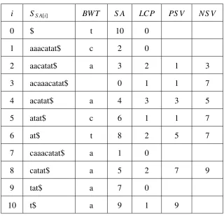
Table 2.3: Suffix array of the stringS = acaaacatatwith LCP: Longest Common Prefix, BWT: BurrowsWheeler transform, SA: Suffix Array, ISA: Inverse Suffix Array, child table and suffix link tables.

childtab suflink

i SS A[i] BWT S A LCP ISA up down next`Index l r

0 $ t 10 0 3

1 aaacatat$ c 2 0 7 3 7

2 aacatat$ a 3 2 1 1 6

3 acaaacatat$ 0 1 2 2 4 5 0 10

4 acatat$ a 4 3 4 7 8

5 atat$ c 6 1 8 4 6

6 at$ t 8 2 5 9 10

7 caaacatat$ a 1 0 9 3 8 9

8 catat$ a 5 2 6 1 6

9 tat$ a 7 0 10 8 10

10 t$ a 9 1 0 0 10

Computation of MEMs using Enhanced Suffix Array

One approach of computing MEMs is to create anESAof concatenation of sequencesXandY of lengthmandnrespectively. However, this approach is not space efficient. A space efficient approach is to createESAofXand then MEMs are computed by matching suffixes ofYagainst theESAofX. The following steps describe the MEMs computing algorithm (more details can be found in [2]). A prefix of a string is a substring that occurs at the beginning of a string. A suffix of a string is a substring that occurs at the end of a string. A left maximal match is

the match which cannot be extended in left of each sequence without a mismatch. Similarly, a

right maximal match cannot be extended to the right without a mismatch.

(37)

2. Match all suffixes ofY againstESAofX, starting with the longest suffix.

3. Find lower and upper bounds (i.e.LCPintervals ofXsay [l..r] ) of a longest prefix match of suffixY. All the prefixes found are right maximal.

4. Do a depth first traversal (on the virtual LCP interval tree) of all right maximal LCP intervals found in the previous step. Each time a leaf node is encountered, check if

X[i−1]_, Y[j−1], wherei=S A[l0_],_l0_{is the singleton lcp-interval corresponding to the}

leaf node and jis the current suffix position inY.

5. The match found is longer than minimum MEM length, report it as MEM.

6. Continue with next suffix ofY.

The MEMs computing algorithm using ESA requires much less memory compared to suffix tree implementation in MUMmer. Later, newer approaches were developed to reduce memory

either by compromising runtime performance or by adopting completely new data structures

and algorithms. The approaches are discussed in the following sections.

2.1.4 SparseMEM

Table 2.4: Sparse suffix array of the stringS = acaaacatatwith LCP, and ISA

i SS A[i] S A LCP ISA

0 $ 10 -1 2

1 aaacatat$ 2 0 1

2 acaaacatat$ 0 1 3

3 acatat$ 4 3 4

4 atat$ 6 1 5

(38)

In order to reduce the memory footprint of algorithms based on ESA, an approach based on sparse suffix arraywas developed [28]. Thesparse suffix arrayis a text index based on every Kth suffix (K = 1,2, ...,n) of a string. For K = 1, the sparse suffix array acts as a full index based on suffix array.

SparseMEM [28] is a MEMs computing program based on this approach. UnlikeVmatch, SparseMEM does not pre-compute suffix link information. Instead, it is computed whenever required. The suffix link can be computed with the help of the inverse suffix array as follows:

l= IS A[S A[l]/K+1] andr= IS A[S A[r]/K+1]

where l and r are the left and right bounds of the suffix link interval respectively. Note that the suffix link interval may require to be extended in both directions for correct results [3].

The ISA computation requires minor adjustments to account for sparse suffix index. ISA is computed as follows:

IS A[S A[j]/K]= jwhere j=, ...,n/K−1

An example of sparse suffix array and corresponding LCP and ISA values is shown in Table 2.4.

Computation of MEMs using Sparse Suffix Array

Consider two stringsS1andS2and supposeLis the minimum length of MEMs. The following steps describe the MEMs computing algorithm (more details can be found in [28]):

1. Create a sparse suffix array of stringS1.

(39)

positions andeandrare the end positions of lcp-intervals respectively. Sinceq: [l..r] is a subinterval ofd : [s..e], therefores≤l,r≤ eandq≥dholds.

3. The right maximal matches are found by un-matching characters from intervalq: [l..r].

(a) The first right maximal match is intervalq: [l..r].

(b) The next interval is the parent lcp-interval of q : [l..r]. Since LCP[l] < q and LCP(r+1)< q, the next lcp-valueq0 = max(LCP[l],LCP[r+1]). The boundary position of the parent interval is obtained by extending interval to the left i.e. l = l−1 untilLCP[l]<q0 and to the right i.e. r=r+1 untilLCP[r+1]<q0.

(c) The expansion continues tillq0 _≥ _d.

4. The right maximal matches found in the previous step are now checked for left

maximal-ity. Since the index is sparse by a factor ofK, all the left maximal matches are found by scanning upto K characters to the left of the right maximal matches.

5. Advance to the next suffix ofS2and continue the matching process.

In the last step of the algorithm, suffix link can be used to find the initial lcp-intervals for

the next suffix position. This is referred assuffix link accelerationin SparseMEM algorithm.

Parallelization technique in sparseMEM

The suffix link acceleration works best with smaller values of K. Note that for an index based on sparse suffix array, moving one suffix position is equivalent to movingKcharacter positions in the string. In step 5 of the previous algorithm, suffix link can only be used if matching for all

0 toK −1 positions in string S2is complete. Due to this limitation, improvement from suffix link acceleration starts to diminish for larger values ofK.

The performance drop due to increase in sparseness factor is addressed by introducing the

concept of parallelization. SparseMEM uses an obvious approach for parallelization which

(40)

stringS2, a process is spawned on a separate processor. The results from theseKprocesses are combined before suffix link acceleration is used for moving to the next suffix position.

2.1.5 EssaMEM

An enhanced version of sparse suffix array data structure which includessparse child arrayis calledEnhanced Sparse Suffix Array (ESSA). EssaMEM [59] is a MEM computation program based onESSAwhich is faster in practice than sparseMEM with the same memory footprint. The essaMEM program proposes two major improvements over the sparseMEM program

dis-cussed in the previous section. They are:

1. The addition of sparse child array which allows the traversal of virtual sparse suffix tree

in constant time.

2. A newskipparameters, which introduces sparseness in query sequence.

The construction of sparse child array remains the same as discussed previously. Typically,

any compressed SA based approach for computing MEMs involves two phases - finding right

maximal matches and then extending these right maximal matches to the left for finding left

maximal matches. The second phase is usually much faster than the first phase. Based on this

observation, the skipparametersis introduced, that increases the work of second phase while decreases the work of first phase by a factor of s. This is achieved by finding right maximal matches of minimum lengthL−s.K+1 characters, which increases the number of right max-imal suffixes. The left maximality is checked for s.K characters to ensure that all the MEMs are larger than lengthL.

(41)

The skip parameter does not work well with simulated sparse suffix links, which are suffix links forESSA. Combination of the two requires a mechanism of controlling sparseness factor K for suffix links along with skipparameters of query sequence. This has not been tried out and therefore when suffix links are used, theskipparametersis set to 1.

The MEMs computation algorithm for essaMEM is same as that of sparseMEM, with the two

enhancements discussed above.

2.1.6 BackwardMEM

The algorithms discussed so far used indexing techniques to search strings in forward direction.

The backwardMEM [46] algorithm uses a data structure which allows searching in backward

direction. The data structure used for indexing in backwardMEM is calledFM-indexand it is discussed in section 2.1.1. A typical backwardSearch algorithm is shown in Algorithm 2.1.1.

The interval [i..j] corresponds to the currently matched string in suffix array. The characterpis the next character in backward search and the new interval is obtained using backwardSearch

algorithm.

Algorithm 2.1.1: backwardSearch(p,[i..j])

i←C[p]+Occ(p,i−1) j←C[p]+Occ(p, j)−1 ifi≤ j

(42)

Computing Parent Intervals

ThebackwardSearchalgorithm generates right maximal matches for a given position in query string. The right maximal matches found correspond to an lcp-interval in a virtual lcp-interval

tree. To find the next right maximal match, backwardMEM program stores two tables,previous smaller values (PSV)andnext smaller values (NSV).

The PSV and NSV table entries are computed as follows:

PS V[i]=max{k|0≤k< iandLCP[k]< LCP[i]} NS V[i]=min{k|i<k ≤nandLCP[k]< LCP[i]}

Once the PS V and NS V information is stored as part of the data structure, the parent interval for an lcp-interval [i..j] withLCP[i]= pandLCP[j+1]=qis determined as:

parent([i..j])=

          

p−[PS V[i]..NS V[i]−1 if p≥q q−[PS V[j+1]..NS V[j+1]−1] if p<q

(43)

Table 2.5: PS V andNS Vtables of the stringS =acaaacatat.

i SS A[i] BWT S A LCP PS V NS V

0 $ t 10 0

1 aaacatat$ c 2 0

2 aacatat$ a 3 2 1 3

3 acaaacatat$ 0 1 1 7

4 acatat$ a 4 3 3 5

5 atat$ c 6 1 1 7

6 at$ t 8 2 5 7

7 caaacatat$ a 1 0

8 catat$ a 5 2 7 9

9 tat$ a 7 0

10 t$ a 9 1 9

Computation of MEMs using the FM-index

Consider two stringsS1andS2and supposeLis the minimum length of MEMs. The following steps describe the MEMs computing algorithm:

1. Create an FM-index data structure of stringS1.

2. Start with the right most character of string S2. Use backwardSearch algorithm for finding right maximal matches of length ≥ L. The right maximal match is a triplet (q,[l..r],p0₂), whereqis the length of the match, [l..r] is the left and right bounds in suf-fix array and p0₂ is the position in S2 for this match. The current match in stringS2 is indicated by the length p0

2+q−1.

3. For each triplet (q,[l..r],p0₂) andq≥ L,

(44)

(b) If left maximal, report MEM.

(c) Find parent interval of (q,[l..r]). Continue untilq≥ Lfor parent interval.

4. Continue with the current position in stringS2.

In order to get a smaller memory footprint, the FM-index (LF−mapping) is stored in a

wavelet tree [60]. A wavelet tree is a data structure which stores sequences in compressed

form. Note that it is not necessary to store BWT, which is only required during left maximal comparison. This is because the wavelet tree allows to access LF−mapping without it, and we have BWT[k] , p if and only if LF(k) < [i..j], where [i..j] is the current p−interval (e.g., backwardsearch(p, [1..n]) returns [i..j]). This is same as replacing the test BWT[k] , S2[p0

2−1] with the testLF(k)<[i..j], where [i..j] is theS2[p

0

2−1]−interval.

Compressed Suffix Array implementation

BackwardMEMalso supports a version of program based oncompressed suffix array. There is a difference between a compressed suffix array and a sparse suffix array - a compressed suffix

array stores each kth _{entry of the su}ffi_{x array} _S_{1 while a sparse su}ffi_{x array stores each} _Kth

suffix ofS1.

The obvious advantage of compressed suffix array is a smaller memory footprint. This is

further reduced by storing the compressed suffix array in a wavelet tree which requires only

(nlogn)/kbits, wherenis length of stringS1 andk is the compress parameter. The size and access time for compressed suffix array depends on compress parameter k ≥ 1. For k = 1, the compressed suffix array acts as a full suffix array and the access time is constant. For

k > 1, everykth_{entry of su}ffi_{x array is stored and the remaining entries are constructed in}_k/₂

(45)

2.1.7 SlaMEM

The MEMs computing programslaMEM [21] is an improvement to the data structures used in BackwardMEM [46]. There is no difference in MEMs computing algorithm as far as the logical steps are concerned. Instead, new remodeled data structures have been proposed for

improving runtime performance and reducing the memory footprint. The improvements are

based on following observations:

1. LCP array is accessed most frequently for resolving parent intervals. A fast mechanism

of retrieving lcp-values helps in improving the performance.

2. To compute the parent intervals, only boundary lcp-values are needed. Having only

boundary lcp-values reduces the memory footprint.

Sampled LCP Array

Based on the above observations, slaMEM samples only boundary values for the LCP array. The PSV and NSV arrays are also computed for these sampled LCP positions. The boundary

positions are sampled as follows:

T opCorners={i: (i+1)_, nandLCP[i]<LCP[i+1]} BottomCorners={i: (i+1)=norLCP[i]> LCP[i+1]}

where T opCorners and BottomCorners represent the boundary positions of lcp-interval corresponding to a BWT string.

Sampled Smaller Values

(46)

S S V[i0]= PS V[i], ifS S V[i0]<i S S V[i0]= NS V[i+1]−1, ifS S V[i0]>i

where i0 is the number of sampled positions in the interval [0,(i−1)] because S S V does not have the same size asPS V/NS V.

It is possible to have overlapping left or right interval positions for two or more intervals.

In such cases, the S S V[i] will store the left or right most parent interval of the overlapping positions. The missing intervals are found by a scan of closest top or bottom corners around

that position. Since the SLCP is sampled, the search is much faster than using full LCP array.

2.1.8 Comparison

Table 2.6 summarizes the important differences and similarities among the applications

dis-cussed in this text. The memory requirement of each tool is shown in terms of bytes per

char-acter. TheK andkare sparseness factor and compress parameter respectively. Once the index is created, each of these algorithms can find MEMs in theoretical time complexity proportional

(47)

Table 2.6: A nutshell comparison of applications. Notations used in the table: ST (Suffix Tree); ESA (Enhanced Suffix Array); SSA (Sparse Suffix Array); ESSA (Enhanced Sparse Suffix Array); LCP (Longest Common Prefix); CT (Child Table); BS (Binary Search).

MUMmer Vmatch sparseMEM essaMEM backwardMEM slaMEM

Text Index ST ESA SSA ESSA FM-index FM-index

Parallelization Yes No Yes No No No

Initial Search ST LCP

CT BS LCP CT Count & Occ Tab Count & Occ Tab

Suffix Link Yes Yes Yes No No No

Memory (bytes)

17n 10n (9/K+1)n (9/K+1)n (4/k+2)n 2.2n

Flexibility

(Memory vs Time)

No No Yes Yes Yes No

Search Order Forward Forward Forward Forward Backward Backward

Commercial open source closed source open source open source open source open source

2.2 E-MEM algorithm

As discussed in previous sections, a typical MEM computation algorithm creates an index

of the reference sequence, which is used for quickly finding seed matches. The seeds are

then extended to find a possible MEM. Depending on the indexing technique, the extension

of seeds may or may not use the index during the extension phase. E-MEM is designed by

using an efficient implementation of simple algorithmic ideas. The algorithm creates an index

based on double hashing which stores k-mers and its positions in the reference. All query k-mers are matched against this index. The matches are extended while ensuring that any k-mer matches resulting in a previously discovered MEM are discarded. E-MEM does not rely

on the index during the extension phase. A high-level overview of the E-MEM algorithm is

provided in Algorithm 2.2.1. The algorithm requires three mandatory input parameters - a

(48)

in Section 2.9. The default value of this parameter is set to one, which means no splitting is

performed and full genomes are used. The input sequences are required to be in FASTA format.

FASTA [37] is a text based format for representing DNA sequences in which nucleotides are represented by a single character codes. It also allows the sequence names and comments to

precede the sequences. Anexact matchbetween two sequencesRandQis a triple (len,s1,s2) such that len ≥ minL, s1 ∈ [0,|R| − len], s2 ∈ [0,|Q| − len], and R[s1..s1 + len − 1] = Q[s2..s2+len−1]. An exact match isleft maximalifR[s1−1]_, Q[s2−1] and right maximal ifR[s1+len]_, Q[s2+len]. Amaximal exact match (MEM )is a left and right maximal exact match.

The algorithm starts by encoding and hashing the reference sequence R. The hash table size is kept roughly two times the number ofk-mersin the sequences. The number of k-mers is estimated based on an approximation which uses total number of base pairs in reference, the

k-mersize and minimum MEM lengthminL . Next, a query sequenceQis encoded and then iterated over for a possiblek-mermatch in the reference hash. If a queryk-mermatch is found in the hash table for the reference, thisk-meris extended, both in left and right direction until a mismatch is encountered. If the length of the match is greater thanminL, the match is reported as a MEM. The E-MEM program can run in serial and parallel mode. The parallelization is

done using OpenMP directives. The algorithm 2.2.1 uses a CurrMEM (linked list) - to keep

(49)

Algorithm 2.2.1: E-MEM(R,Q,minL)

comment:Input - two sequences R and Q and a minimum MEM length minL

Choose a division factor D

Split R intoR1,R2, ...,RD; Split Q intoQ1,Q2, ...,QD

comment:Splitting details discussed in Section 2.9

fori←1toD

do                                                                                                                                                                           

EncodeRi

comment:Encoding discussed in Section 2.3

l←minL−k+1

comment:kisk−mersize

while(l<=|Ri| −k+1)

do           

Hash thek−merat positionlofRi

l←l+minL−k+1

for j←1toD

do                                                                                         

EncodeQj

forl←1to|Qj| −k+1)

do                                                                       

Get thek−mer qat positionlinQj

Search fork−mers r=qin the hash table ofRi

forEach occurrence ofrwith extension>=minL

do                                      Check CurrMEMs

if((q,r) discovers a new MEM)

then if(MEM at ends ofRiorQj)

thenAdd to MEMext

elseAdd to file (by start position inQj)

Update CurrMEMs

Remove Hash table forRi

Process MEMext to extend MEMs

Move MEMs from MEMext to appropriate files

forEach file with MEMs

do           

Sort MEMs by position in Q

Remove duplicates

(50)

2.3 Sequence Storage

The E-MEM program uses many techniques to reduce memory and improve performance. To

reduce memory requirements, the sequences are read from FASTA files and stored in a 2-bit

encoding scheme. All four nucleotides can be represented with 2-bits as{A=00, C=01, G=10,

T=11}. The storing of a nucleotide in 2-bits instead of a byte reduces memory requirement by

a factor of 4. An array of unsigned 64-bit integers is used to store the entire genome with a

single unsigned 64-bit holding 32 nucleotides. The genome sequence containing base pair N

(an ambiguous base) are replaced with a random nucleotide and the position is tracked for final

MEM reporting. The details of unknown base handling are discussed in Section 2.8.

2.4 E

ffi

cient

k-mer Storage

We observed that storing all k-mers in the reference sequence is unnecessary as it leads to redundant MEM discovery. To avoid redundant hits, k-mers are stored at intervals of length minL −k + 1, where minL is minimum MEM length and k is the k-mer size. This ensures that at least onek-mer is stored in any possible MEM of lengthminL. Figure 2.3 shows three consecutive positions for k-mer hashing. It is clearly seen that storing k-mers at an interval reduces memory requirement and processing time for hashing. It also avoids redundant hits

during later stages, which results in significant performance improvements.

(51)

2.5 Hash Table and hashing function

The E-MEM algorithm uses hashing to efficiently store and search k-mers for matching be-tween query and reference sequences. The technique involves creation of an associate array

abstract data structure, calledhash table. A hash table uses ahash functionto compute an in-dex which locates the desired value. The average time complexity ofinsert, deleteandsearch operation isO(1) which makes hashing a very efficient data structure.

The input to E-MEM hashing function is an unsigned value obtained from 2-bit

represen-tation of k-mers. The hash function then computes a modulus of input value with the size of the hash table, which is used as an index in the hash table. The hash table size is a prime

num-ber to ensure that all indexes are probed. It is possible that hash function maps two different

k-mer values to same index in the hash table. This is calledcollisionand over the years many techniques are developed to deal with collision in hashing algorithms. A popular method for

collision resolution in hash tables is calledOpen Addressing. In this method, the collisions are resolved by searching through alternate locations in hash table until either the key is found or

an unused location is found, which indicates that the key does not exist in the hash table. The

three most common open addressing approaches are Linear Probing, Quadratic Probingand Double Hashing. The objective of any good hashing technique is to distribute the keys evenly to avoid collisions while maintaining constant time performance of basic operations.

E-MEM uses double hashing technique for efficient storage and retrieval ofk-mer values. The load factor is kept under 50% to maintain high performance. At each index in the hash

table where ak-mer maps, a list of reference position are stored. The positions are maintained in an array which grows in powers of 2. The first position in the array stores the number of

reference positions in the array. The array grows dynamically as it becomes full and space is

(52)

2.6 Searching query

Storing all k-mers in the reference sequence is not necessary, as mentioned in Section 2.4 however all k-mers in the query sequence have to be considered. For every query k-mer, all matching k-mer positions in the reference are investigated for a possible MEM. An efficient implementation is achieved by performing bit level operations. A 64-bit sliding window is

used to read query sequence and a bit mask of 2k 1’s extracts the k-mer bits. Moving the sliding window by 2 bits to the right gives the nextk-mer in the query sequence. To maintain an efficient sliding operation, a byte (8 bits) is shifted each time instead of two bits. This

restricts the maxk-mer size to 28 nucleotides.

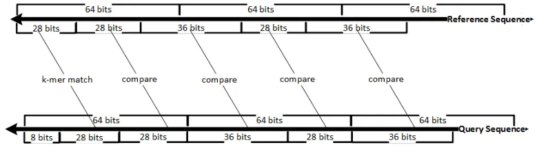
Once ak-mer hit between query and reference is found, it needs to be extended efficiently in both directions for a possible MEM. Extending one character at a time will result in a very

inefficient algorithm. Since the sequences are stored in blocks of 64 bits, comparisons are

performed using very few bit operations as shown in Figure 2.4.

Figure 2.4: Efficient k-mer matching

For example, Figure 2.4 shows a k-mer match of size 14 or 28-bits found between query and reference sequence. Next, the extension is performed by matching the query sequence in

2 blocks of 28 and 36 bits. A 64-bit block is compared using two comparison operations and

(53)

2.7 Handling redundant MEM matches

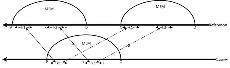
The E-MEM program uses many techniques to make it more efficient. The algorithm extends

initial k-mer hits between query and reference sequences to find a MEM. Since every k-mer in the query sequence is looked up in the reference hash, it is expected that a MEM longer

than minimum MEM lengthminL is discovered by at least twok-mers. The secondk-mer hit simply rediscovers the previously found MEM. Figure 2.5 shows a possible scenario for one

such case. It is important that all such cases are discovered quickly and discarded for efficient

functioning of the E-MEM program.

Figure 2.5: Redundant MEMs

The E-MEM algorithm avoids redundant computation of MEMs by keeping track of the

relative distance of the currentk-mer position with respect to the already discovered MEMs in the query sequence. The relative distance thus obtained is used with the currentk-mer position in the reference sequence to compute MEM coordinates. If the computed MEM coordinates