The Effects of Intraspecific Competition and Stabilizing Selection on a Polygenic Trait



DOI: 10.1534/genetics.103.018986

The Effects of Intraspecific Competition and Stabilizing

Selection on a Polygenic Trait

Reinhard Bu

¨rger*

and Alexander Gimelfarb

*Department of Mathematics, University of Vienna, A-1090 Vienna, Austria and†_{Department of Genetics,} Stanford University, Stanford, California 94305

Manuscript received June 16, 2003 Accepted for publication December 31, 2003

ABSTRACT

The equilibrium properties of an additive multilocus model of a quantitative trait under frequency- and density-dependent selection are investigated. Two opposing evolutionary forces are assumed to act: (i) stabilizing selection on the trait, which favors genotypes with an intermediate phenotype, and (ii) intraspe-cific competition mediated by that trait, which favors genotypes whose effect on the trait deviates most from that of the prevailing genotypes. Accordingly, fitnesses of genotypes have a frequency-independent component describing stabilizing selection and a frequency- and density-dependent component modeling competition. We study how the equilibrium structure, in particular, number, degree of polymorphism, and genetic variance of stable equilibria, is affected by the strength of frequency dependence, and what role the number of loci, the amount of recombination, and the demographic parameters play. To this end, we employ a statistical and numerical approach, complemented by analytical results, and explore how the equilibrium properties averaged over a large number of genetic systems with a given number of loci and average amount of recombination depend on the ecological and demographic parameters. We identify two parameter regions with a transitory region in between, in which the equilibrium properties of genetic systems are distinctively different. These regions depend on the strength of frequency dependence relative to pure stabilizing selection and on the demographic parameters, but not on the number of loci or the amount of recombination. We further study the shape of the fitness function observed at equilibrium and the extent to which the dynamics in this model are adaptive, and we present examples of equilibrium distributions of genotypic values under strong frequency dependence. Consequences for the maintenance of genetic variation, the detection of disruptive selection, and models of sympatric speciation are discussed.

M

Typ-dependence as a major factor in maintaining non-synon-ical situations leading to such selection include attacks

ymous polymorphisms seems overwhelming.” However, of parasites, presence of predators or competitors,

re-he also stresses tre-he importance of more empirical work source utilization, sexual dimorphism, and behavioral

needed to discriminate between FDS and other forms variability. Although it has been long known among

of balancing selection. Often, however, FDS will interact population geneticists that frequency-dependent

selec-with other forms of selection, or act in addition to them, tion (FDS) can maintain genetic polymorphism much

frequently on quantitative traits (e.g., Bulmer 1974, easier than frequency-independent selection (e.g.,Wright

1980;Slatkin1979;Clarkeet al.1988). In such cases, 1969; Cockerham et al. 1972; Matessi and Jayakar

an evaluation of the importance of FDS in maintaining

1976; Clarke 1979; Christiansen and Loeschcke

genetic variation relative to selective pressures that are 1980;Asmussen1983;AsmussenandBasnayake1990),

likely to be frequency independent, such as many caused even some pioneers in studying the evolutionary

signifi-by the abiotic environment or arising from the require-cance of frequency dependence (FD) are skeptical

ments of a functional morphology and developmental whether FD is responsible for a large fraction of

ob-and physiological constraints, may be particularly diffi-served polymorphisms (Maynard Smith1998). In

con-cult. One reason is that the determination of the kind and strength of selection acting on a (set of) trait(s) is everything but straightforward (e.g.,LandeandArnold This article is dedicated to the memory of Sasha Gimelfarb, who _{1983;Endler1986;Schluter1988;Kingsolveret al.} died May 11, 2004.

2001). Second, the majority of theoretical studies of the

1_{Corresponding author:Institut fu¨ r Mathematik, Universita¨t Wien,}

evolutionary consequences of FDS either ignore genetics Strudlhofgasse 4, A-1090 Wien, Austria.

E-mail: [email protected] (e.g., evolutionary game theory and the so-called adaptive

dynamics approach) or are based on very simple genetic tion by showing that if the strength of competition rela-tive to stabilizing selection exceeds a certain threshold, models (a single locus or a normally distributed trait with

given variance). Therefore, little is known about the pat- the trait is under disruptive selection; hence genetic variance should be maintained. Otherwise, the trait is terns of genetic variation maintained by FDS.

General and systematic treatments of genetic models under stabilizing selection, which usually depletes heri-table variation (see also thediscussion). However, ques-with frequency- and density-dependent selection are

available only for a single locus (Nagylaki1979;Asmus- tions concerning the extent of variation maintained by FDS or if and how conclusions depend on the underly-sen 1983; Asmussen and Basnayake 1990). In these

models, fitnesses are assigned directly to genotypes, ing genetic structure can be answered only on the basis of more explicit genetic models.

though in a rather general way. These and other

investi-gations clearly demonstrate that FDS may strongly in- We complement and extend previous studies in sev-eral directions. First, we admit multiple diallelic loci to fluence the genetic structure of a population and has a

much higher potential in maintaining genetic variation contribute (additively) to the trait. Second, the popula-tion size is allowed to change according to its demo-than frequency-independent selection. In addition,

al-ready for one-locus two-allele models in which genotypic graphic dynamics. Because random genetic drift is ig-nored, the dynamics are still deterministic. Third, fitnesses are linear functions of the genotype

frequen-cies, complex dynamic behavior, such as chaos, may occur stabilizing selection that is asymmetric with respect to the existing range of phenotypic values is explored. for relatively wide ranges of parameter values (Altenberg

1991;GavriletsandHastings1995). Fourth, to cover a wide range of parameters, in

particu-lar from the high-dimensional genetic parameter space, We pursue a different approach by making specific

assumptions on how selection acts on phenotypes. In do- we adopt the statistical and numerical approach of Bu¨ rgerandGimelfarb(1999, 2002). Thus, for a given ing so, we lose generality compared to some of the

single-locus studies. However, it enables us to tackle questions number of loci, a range of recombination rates, and given ecological and demographic parameters, we calcu-such as, How strong must FD be relative to other selective

forces, such as stabilizing selection, to have a noticeable late the quantities of interest by iterating a large number of genetic systems with randomly chosen locus effects impact on the genetic structure of a population? or, When

is FD strong enough to be phenotypically detectable? To and initial conditions until equilibrium is reached and then computing the appropriate averages. This numeri-this end, we consider a quantitative trait that is subject to

(frequency-independent) stabilizing selection and medi- cal approach is complemented by analytical results and allows us to derive general inferences on the patterns ates frequency- and density-dependent selection through

intraspecific competition;i.e., individuals of similar phe- of genetic variation resulting from the interaction of multilocus genetics with FDS. In particular, the strength notypes compete. We use a functional form for fitness

of the trait introduced by Bulmer (1974, 1980) that of FD that leads to highly polymorphic genetic systems and to disruptive selection is determined. Also the evolu-does not specify the causes of stabilizing selection,i.e.,

whether real or induced by pleiotropic effects. Never- tion of mean fitness and of the equilibrium distribution of genotypic values under strong FD is examined. theless, mathematically this model is closely related to

models based on differential resource utilization and a This is not the first multilocus study exploring the amount of genetic variation maintained by FDS on a Lotka-Volterra approach (Slatkin1979;Christiansen

and Loeschcke 1980; Loeschcke andChristiansen quantitative trait.Clarkeet al.(1988) andManiet al.

(1990) employed a model of selection that is similar to 1984). Previous studies of this type of model assumed

a single locus contributing to a normally distributed Bulmer’s (1980), but differs in the way competition and stabilizing selection are modeled. Moreover, they trait (Bulmer 1974, 1980; Slatkin 1979), a classical

quantitative-genetics approach for a normally distrib- assume a finite population and admit several multiallelic loci with recurrent mutation. Their results are purely uted trait (Slatkin1979), a single locus with multiple

alleles (Christiansen and Loeschcke 1980), or two numerical and the main focus is on variation at the gene level. Therefore, direct comparison with the models recombining diallelic loci contributing additively to a

quantitative trait without assumptions on its distribution discussed above is difficult. The purpose of our study is not to demonstrate that FDS can be important, but (LoeschckeandChristiansen1984;Bu¨ rger2002a,b).

Roughly, conditions were identified under which FD is rather to identify conditions under which it has signifi-cant effects on the genetic structure of a population, strong enough to induce disruptive selection and

main-tain polymorphism. In the two-locus models, the amount what and how large these effects are, and how genetical and ecological parameters interact.

of genetic variation and the possible equilibrium pat-terns and their dependence on the parameters were derived.

THE MODEL Studies with simple genetics (Bulmer 1974, 1980;

varia-sufficiently large to ignore random genetic drift. Selec- specific competition function␣P(g), which measures the strength of competition experienced by phenotypegif tion acts only through differential viabilities. Individual

fitness is assumed to be determined by two components: the population distribution isP, is given by

(i) by stabilizing selection on a quantitative character _␣

P(g)⫽

兺

␣(g,h)P(h) and (ii) by competition among individuals. The trait is

determined byn additive, diallelic loci of arbitrary

ef-and calculated to be fect. The model is an extension of that used inBu¨ rger

(2002b).

␣P(g)⫽1⫺ 1 2V␣

[(g⫺g)2⫹_V

A] . (3)

Ecological assumptions: The first fitness component is frequency independent and may reflect some sort

Here,gandVAdenote the mean and (additive genetic)

of direct selection on the trait, for example, through

variance, respectively, of the distributionPof genotypic differential supply of a resource whose utilization

effi-values. ciency is phenotype dependent. However,

frequency-Similar toBulmer’s (1974, 1980) model, we assume independent stabilizing selection could as well be

that the absolute fitness of an individual with genotypic caused by indirect selection through pleiotropic side

value (phenotype)gis given by effects of alleles that contribute primarily to

fitness-related traits (e.g., Robertson 1967; Keightley and

W(g)⫽

冢

冣

environ-mental variation and deal directly with the fitnesses of

where␳ and ␬are positive parameters and N denotes genotypic values. In the absence of

genotype-environ-the total population size. For notational simplicity, genotype-environ-the ment interaction, this is no restriction because in the

dependence of W(g) on N and P is omitted. In the present model the only effect of including

environmen-context of density-dependent growth models, the pa-tal variance was a deflation of the selection intensity.

rameter ␳ in (4) is related to the growth rate of the For simplicity, we sometimes use the words genotypic

population and␬is proportional to the carrying capac-value and phenotype synonymously.

ity. More precisely, in a monomorphic population in Stabilizing selection is modeled by the quadratic

func-whichg⫽ g⫽ ␪andVA⫽0, the fitness (of the

popula-tion

tion) becomes␳ ⫺N/␬; hence the carrying capacity is

S(g)⫽1⫺(g⫺ ␪)

2

2Vs

, (1)

K⫽ ␬(␳ ⫺1) . (5)

Our model of FDS is closely related to models that whereVsis an inverse measure for the strength of

stabiliz-are based on Lotka-Volterra equations (Slatkin1979; ing selection and␪ is the position of the optimum. Of

Christiansenand Loeschcke 1980; Loeschcke and course, S(g) is assumed to be positive on the range

Christiansen1984). The relation between these mod-of possible phenotypes, thus restricting the admissible

els and ours is worked out inBu¨ rger(2002b), where values ofVs. We use a scale on which the range of possible

it is shown that all these ecological models lead to fitness phenotypes is the interval [0, 1] (seeGenetic assumptions

functions that are mathematically equivalent to first or-below). Hence, if␪ ⱖ0.5, thenVsmust satisfyVsⱖ1⁄2␪2.

der in 1/Vsand 1/V␣. Thus, for sufficiently weak overall

We exclude pure directional selection by assuming 0⬍

selection, the differences vanish. As explained in

␪ ⬍1.

Bu¨ rger(2002b), the present choice of the fitness func-The second component of fitness is FD. We assume

tion makes the model more easily amenable to mathe-that competition between phenotypes gand h can be

matical analysis and does not lead to certain special described by

effects that a Gaussian fitness function causes under strong selection. If stabilizing selection is modeled by a

␣(g,h)⫽ 1⫺ 1

2V␣(g⫺h)

2_{, (2)}

Gaussian fitness function, the equilibrium structure is much more complex than with quadratic fitness. This with the obvious constraint that the maximum differ- is so in the absence of FD (Nagylaki1989; Willens-ence between genotypic values must be no larger than dorfer and Bu¨ rger 2003) as well as for very strong FD (LoeschckeandChristiansen1984). Our fitness

√

implies that competition between individuals of similar function is also closely related to that ofMatessiet al.

(2001); if higher-order terms are omitted, the induced phenotypes is much stronger than that between

individ-uals of very different phenotypes, as will be the case if dynamics and equilibrium structure become equivalent. Genetic assumptions: The trait values g are deter-different phenotypes preferentially utilize deter-different

food resources. Small V␣ implies a strong frequency- mined additively byn diallelic loci. There is no domi-nance or epistasis. The contribution of one allele at dependent effect of competition, whereas in the limit

V␣→ ∞, FD vanishes. LetP(h) denote the relative fre- each locus ᐉ is zero, and the contribution, ␤ᐉ, of the

intra-It is assumed that the minimum and maximum geno- plicit and analytical characterization of the equilibrium typic values are always zero and one. Therefore, the properties of multilocus models in terms of all parame-actual contribution by the second allele at locus ᐉ is ters and initial conditions would be of limited value, scaled to be␥ᐉ⫽1⁄2 ␤ᐉ/兺nk⫽1␤k. It follows that the geno- even if it were feasible. Therefore, we use a different typic value of the total heterozygote is always1_⁄

2, and the approach by evaluating the quantities of interest for

average allelic effect among the nloci controlling the many randomly chosen parameter sets and initial condi-trait is␥ ⫽1/(2n). This normalization has the advan- tions and, consequently, obtaining statistical results. tage that the strength of selection on genotypes can be We proceeded as follows. For a given set ofecological

compared for different numbers of contributing loci. parameters (␳,␬,V␣,␪,Vs), a given numbernof loci, and

The effect of an increasing number of loci is a finer a given range of recombination rates, we constructed resolution of possible phenotypes through genotypic _{ⱖ1000 of what we call genetic parameter sets (allelic}

values. _{effects of loci and recombination rates between adjacent}

Dynamics:Gametes are designated byi, their frequen- _{loci from the given range). For each genetic parameter} cies among zygotes in consecutive generations bypiand set, allelic effects were obtained by generating values␤_ᐉ

p⬘i, and the fitness of a zygote consisting of gametes j (ᐉ ⫽ 1, 2, . . . , _n) as independent random variables, and k by Wj k (we do not indicate the frequency and _{uniformly distributed between 0 and 1, and} trans-density dependence). LetR(jk→i) denote the proba- _{forming them into the actual allelic effects, ␥}

ᐉ⫽ 1⁄2␤ᐉ/

bility that a randomly chosen gamete produced by ajk _兺

k␤k. The additivity assumption yields the genotypic val-individual is i. The function R is determined by the _{ues, and from Equations 1, 3, and 4, the genotypic} pattern of recombination between loci. Since random _fitnessesW

jkare calculated in each generation. Recombi-mating is assumed and gamete frequencies are mea- _{nation rates between adjacent loci, r}

ᐉ,ᐉ⫹1(ᐉ ⫽ 1, . . . ,

sured after reproduction and before selection, Hardy- _{n⫺1), were either assumed to be all}1_⁄

2or obtained as

Weinberg proportions obtain and the genetic dynamics _{independent random variables, uniformly distributed} can be described in terms of gamete frequencies by the _{between 0 and 0.01. We assumed absence of}

interfer-well-known system of recursion relations _{ence and refer to these two scenarios as free}

recombina-tion and tight linkage, respectively.

p⬘i ⫽W⫺1

兺

WjkpjpkR(j k→i) , (6)

For each of such constructed genetic parameter sets, the recursion relations (6) and (7) were numerically whereW⫽兺j,kWjkpjpkis the mean fitness (e.g.,Bu¨ rger

iterated starting from 10 different randomly chosen ini-2000).

tial gamete distributions. To make the initial distribu-The ecological dynamics follow the standard

re-tions more evenly distributed in the gamete state space, cursion

they were chosen such that the (Euclidean) distance

N⬘ ⫽N W. (7) _{between any two of them was no less than a}

predeter-mined value (0.25, 0.30, and 0.35 for two, three, and Thus, for a genetically monomorphic population with

four loci, respectively). An iteration was stopped after

g⫽g⫽ ␪ and VA ⫽ 0, the classical discrete logistic

generation t when either an equilibrium was reached equation is obtained, N⬘ ⫽ N(␳ ⫺ N/␬). As is well

(in the sense that the geometric distance between gamete known, monotone convergence to the carrying capacity

distributions in two consecutive generations was⬍10⫺12_),

K⫽ ␬(␳ ⫺1) occurs if and only if␳ ⱕ2 and oscillatory

ortexceeded 106_{generations (in some cases even 10}7_).

convergence occurs if 2⬍ ␳ ⱕ 3 (e.g., Bu¨ rger2000).

If equilibrium was not reached, the parameter combina-Throughout this study, we are concerned only with

suf-tion was excluded from the analysis. Usually, the propor-ficiently small values ␳so that the ecological dynamics

tion of excluded runs was small enough not to introduce are simple; i.e., convergence to a unique equilibrium

a bias. In a small region of ecological parameters (the population size occurs. Also the initialN0 was chosen

so-called transitory region, see next section), extremely sufficiently small (except for exploratory reasons,N0⫽

slow convergence was the rule because of very flat fitness

K) so that population size always remained positive.

landscapes. Since for some parameter combinations in Because this study is devoted to the equilibrium

struc-ture and the equilibrium population size is uniquely this region onlyⵑ20% of the runs converged within 106

determined if␳ ⱕ3, this choice ofN0is no restriction. generations, we stopped runs that had not converged

only after 107_{generations. At that time}ⵑ_{90% had}

ful-filled our convergence criterion. If convergence within THE STATISTICAL APPROACH _{the specified maximum number of generations did not}

occur, it was because of extremely slow convergence of Usually, parameters of genetic systems controlling

allele frequencies. Apart from a very flat fitness function, quantitative traits are unknown or can be inferred only

the main reason for slow convergence was the presence indirectly. Since, in addition, the dimensionality of the

of alleles of extremely small effect. No instance of com-parameter space and the number of gametes and

For each parameter combination withnⱕ4 loci, all ecological parameters, number of loci, and recombina-tion scenario. The data presented in the figures and statistics are based on 1000 genetic parameter sets that

led to equilibration; forn ⫽ 5 loci they are based on tables are such averages. We denote the average over

VrbyVrand refer to it as the relative genetic variance.

500 such genetic parameter sets. For each parameter

set we calculated the number of different equilibria, Its use is preferable when comparing systems with differ-ent numbers of loci, because the variance itself is the gamete frequencies at each equilibrium, and the

number of trajectories (initial distributions) converging strongly dependent on the average effect among loci, which decreases in proportion to 1/(2n). For a given to each equilibrium. Using this database, the

equilib-rium properties were analyzed. Whenever we use the number of loci, the relative genetic varianceVrand the

(average) genetic varianceVAbehave very similarly (results

term equilibrium without qualification, we mean a

(lo-cally asymptoti(lo-cally) stable equilibrium, unless other- not shown). BecauseVmax⫽1⁄2

兺

wise mentioned. in principle the whole distribution) ofVmaxcan be

calcu-Most of our numerical results are for two, three, and lated for each n. For n ⫽ 2, 3, 4, we have E[Vmax]⫽

four loci; only a few are for five or more because some 1_⁄

4(1⫺ ln 2) ⬇0.077, 1⁄4(1⫹ 6 ln 2⫺ 9⁄2ln 3)⬇ 0.054,

four- and most five-locus parameter combinations are and1_⁄

4(1⫺ 44 ln 2⫹27 ln 3)⬇0.041, respectively.

Mul-extremely time consuming. With five loci, for instance, tiplyingVrbyE[Vmax] yields an estimate ofVAthat

typi-1600 generations takeⵑ1 sec on an AMD Athlon proces- cally is within ⵑ10% of the “true” value (results not sor with 1.3 GHz. Since with five loci, typical runs for shown). The polymorphism displayed in the figures is weak or very strong FD equilibrate only after several the average number of polymorphic loci at a stable hundred thousand generations (for intermediate FD equilibrium, the average being taken over all 10 trajecto-more than 10 times as many), 10 initial conditions for ries in all 1000 genetic parameter sets.

each parameter combination are taken, and average For later use we note that for any number of loci we statistics are performed over 500 genetic parameter sets, haveVmaxⱕ 1⁄8, where the maximum is attained if the

the computing time was correspondingly long. The total alleles at one locus have effects 0 and1_⁄

2 and those at

computer time for the project was equivalent to ⵑ2 other loci have no effect, andVAⱕ1⁄8, where the

maxi-CPU years, but we used several computers. mum is attained if there are only the two gametes with

effects 0 and1_⁄

2in the population, each with frequency 1_⁄

2, because zygotes are in Hardy-Weinberg proportions.

PROPERTIES OF GENETIC VARIATION _{For a given number of loci and given recombination} AT EQUILIBRIUM

scenario, the genetic parameter sets as well as the initial In this section, we explore how the genetic variation conditions are the same for all ecological parameter maintained at equilibrium is affected by the strength of sets. Therefore, variation among quantities of interest FD relative to pure stabilizing selection and what role comes almost exclusively from variation in the ecologi-the oecologi-ther parameters in ecologi-the model, such as number of cal parameters. Only the exclusion of slow runs leads loci, recombination rates, position of the optimum, and to slight variation among the genetic parameter sets the demographic parameters, play. For this purpose, we used for different ecological parameter combinations. study the equilibrium properties, i.e., the number of An important role in this article is played by the quan-stable equilibria and their degree of polymorphism, the tity

genetic variance maintained, and the amount of linkage

disequilibrium. _f⫽ Vs

V␣, (8)

For each parameter combination, we recorded the equilibria to which at least 1 of the 10 trajectories

con-which measures the strength of FD,i.e., the strength of verged, their number, the number of trajectories

con-competition relative to stabilizing selection. If f ⫽ 0, verging to a given equilibrium, the number of

polymor-there is no FD, whereasfⰇ1 means strong FD. As we phic loci at each equilibrium, the (additive) genetic

see below, the properties of our model depend on Vs

variance,VA, and the genic variance,VLE (i.e., the

vari-andV␣separately; however, to leading order in 1/Vs(the

ance that would be observed under linkage

equilib-strength of stabilizing selection) and 1/V␣ (the strength rium), at equilibrium. As a measure for global linkage

of competition), they depend only onf. In addition, we disequilibrium, we use the ratioVA/VLE. To facilitate the

introduce the compound demographic parameter comparison of genetic systems with different numbers

of loci, we calculated the ratioVr⫽VA/Vmaxof the genetic

␽ ⫽ ␳␬

N ⫺1 . (9)

variance and the maximum possible variance, Vmax, in

the given genetic system under the assumption of

link-The symmetric case:We begin by discussing numeri-age equilibrium.

cal results for the symmetric case in which the optimum These values were then averaged over all 1000 genetic

␪coincides with the genotypic value of the completely parameter sets, and standard deviations were calculated.

This yielded our “quantities of interest” for each set of heterozygote genotypes, i.e.,␪ ⫽ 1_⁄

is very slightly higher than Vmax (actually, very slowly

increasing as f increases further) and nearly indepen-dent of the number of loci. The average amount of linkage disequilibrium is very small in this case, even for large values of f; i.e., the average VA/VLE is always

⬍1.03 (results not shown). For tight linkage, the genetic variance increases to values much higher thanVmaxasf

increases above 1.0. The increase beyondVmaxis almost

solely due to the build-up of strong positive linkage disequilibrium; the more loci, the higher the linkage disequilibrium. If f ⱖ 1.25, we haveVLE ⫽ Vmax under

both recombination scenarios because then a unique stable, fully polymorphic equilibrium is maintained (see Tables 1 and 2) at which all allele frequencies are 1_⁄

2.

Therefore, our measureVA/VLE for linkage

disequilib-rium equals Vr if FD is strong. For weak or moderate

FD (f⬍1), linkage has only a minor, in general dimin-ishing, effect on the genetic variance (the more loci, the weaker the effect). As under pure stabilizing selection (Bu¨ rgerandGimelfarb1999), not only the (absolute) genetic variance but also the relative variance decreases with increasing number of loci if FD is weak (for some five-locus data see Table 3).

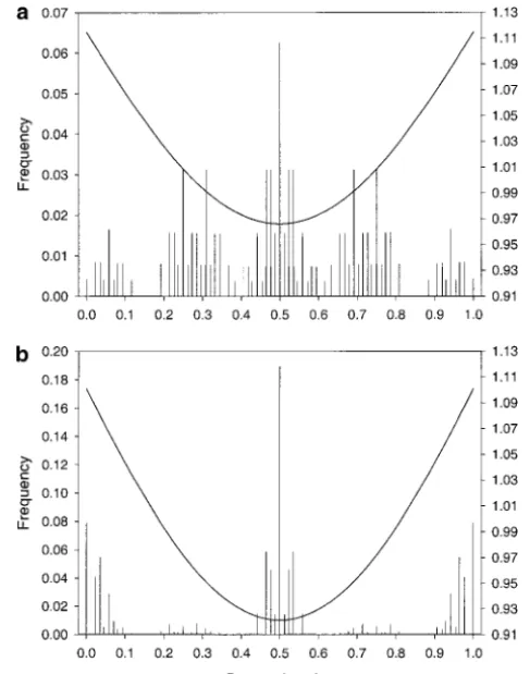
Figure 1b shows that for f ⱖ 1.25 all equilibria are completely polymorphic, irrespective of recombination. They are also unique (Tables 1–3) and, as already noted, symmetric in the sense that all allele frequencies are1_⁄

2.

They differ, of course, in their linkage disequilibria. If Figure1.—Relative genetic variance (a) and polymorphism f ⬍1 and recombination is free, then the average de-(b) as a function off⫽Vs/V␣for n⫽ 2, 3, and 4 loci and gree of polymorphism is⬍1 but steadily increasing and free recombination (solid symbols) as well as tight linkage _{nearly independent of the number of loci. As f} in-(open symbols). The strength of stabilizing selection is fixed

creases beyond 1, a marked increase of polymorphism to (Vs⫽1.25; this reduces the fitness of the extreme genotypic

the maximum possible amount occurs. For tight linkage values by 10%) andV␣is varied [the following pairs (V␣,f)

correspond: (∞, 0), (5.0, 0.25), (2.0, 0.63), (1.5, 0.83), (1.3, andf⬍1, on average equilibria exhibit more polymor-0.96), (1.2, 1.04), (1.0, 1.25), (0.8, 1.56), and (0.5, 2.5)]. In _{phism than for free recombination, and for a range of} addition,␪ ⫽0.5,␳ ⫽2, and␬ ⫽10,000. The bars between _{valuesfthe amount of polymorphism maintained may} a and b indicate the type of fitness function observed for given

even decrease as fincreases. This latter phenomenon

f. The top bar indicates the true fitness function, the bottom

is more pronounced if stabilizing selection is stronger bar its quadratic approximation (see disruptive vs.

stabi-lizing selection). Black indicates stabilizing selection (results not shown) and was demonstrated analytically (傽-shaped); gray, a complicated fitness function (typically _{for two loci (Bu¨ rger2002a,b).}

M-shaped); and light gray, disruptive selection (傼-shaped).

The bars in different shades of gray between the top and bottom of Figure 1 indicate the shape of the fitness function at equilibrium for the corresponding value f

parameters here are␳ ⫽2 and ␬ ⫽10,000. This value

(seedisruptivevs.stabilizing selection). of␳ensures that rapid convergence ofNto the carrying

Tables 1 and 2 provide detailed insights into the ef-capacity occurs. The role of ␳and␬is studied further

fects of increasing FD on the equilibrium structure. For below.

free recombination (Table 1), no stable equilibria with Figure 1 visualizes some of the most important

gen-two or more polymorphic loci were found iff ⬍1. As eral findings. It shows a distinct, threshold-like

depen-Table 1 shows, the introduction of FD leads to a steady dence of the (average) relative genetic variance and the

increase of single-locus polymorphisms at the expense (average) amount of polymorphism on fasfincreases

of stable monomorphic equilibria until a complete re-from values ⬍1.0 to values⬎ ⵑ1.2. This threshold is

structuring of the equilibrium pattern occurs between more pronounced the larger the number of loci is. The

f ⫽ 1 and f ⫽ 1.25. If f ⬎ 1, stable monomorphic genetic variance is slowly, but steadily, increasing with

equilibria cease to exist and as soon asfⱖ 1.25, there

f if f ⬍ 1. Then a rapid increase occurs in a narrow

is a unique stable, fully polymorphic equilibrium. Table interval, and for free recombination the genetic

vari-2 shows that similar behavior occurs with linked loci, the ance nearly levels off as f exceeds ⵑ1.2. For larger

TABLE 1

Equilibrium structure forn⫽2, 3, and 4 loci and free recombination

Two loci Three loci Four loci

Polymorphism Polymorphism Polymorphism

f No. (E) 0 1 2 No. (E) 0 1 2 3 No. (E) 0 1 2 3 4

0.00 2 0.51 0.49 0 2.5⫾1.0 0.52 0.48 0 0 3.7⫾1.6 0.57 0.43 0 0 0

0.25 2 0.38 0.62 0 2.6⫾1.1 0.41 0.59 0 0 3.8⫾1.7 0.44 0.56 0 0 0

0.50 2 0.26 0.74 0 2.7⫾1.2 0.28 0.72 0 0 4.0⫾1.8 0.31 0.69 0 0 0

0.83 2 0.09 0.91 0 2.9⫾1.3 0.10 0.90 0 0 4.3⫾1.9 0.11 0.89 0 0 0

0.96 2 0.03 0.97 0 3.2⫾1.4 0.04 0.96 0 0 4.6⫾1.9 0.03 0.97 0 0 0

1.04 2 0 0.73 0.27 2.8⫾0.9 0 0.65 0.35 0 3.6⫾1.5 0 0.37 0.59 0.04 0.00

1.14 1.1⫾0.3 0 0.07 0.93 1.1⫾0.3 0 0.02 0.07 0.92 1.1⫾0.5 0 0.00 0.00 0 0.99

1.25 1 0 0 1 1 0 0 0 1 1 0 0 0 0 1

1.56 1 0 0 1 1 0 0 0 1 1 0 0 0 0 1

2.50 1 0 0 1 1 0 0 0 1 1 0 0 0 0 1

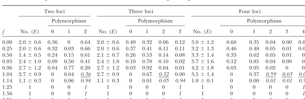
Presented are the average number of equilibria⫾the standard deviation, denoted by No. (E), and the proportion of trajectories converging to an equilibrium with the indicated number of polymorphic loci. Italic type indicates that all equilibria of this type have nonnegative linkage disequilibrium. Underlined italic type indicates that negative and nonnegative linkage disequilibria occur. The following parameters are the same in all cases:␬ ⫽10,000,␳ ⫽2,Vs⫽1.25,␪ ⫽0.5. Data are not shown for all valuesfdisplayed in Figure 1 but, in addition, data for the largest possiblef(f⫽2.5) are included. (Integer entries such as 0, 1, or 2 mean exactly this value,i.e., no variation among the 1000 genetic parameter sets was observed.)

FD, stable equilibria may exist at which two or more loci may exist, whereas for large enough f all equilibria exhibit positive linkage disequilibrium. In the transitory are polymorphic. But again, single-locus polymorphisms

are increasing with increasingfat the expense of stable region, the equilibrium structure may be rather com-plex and several stable equilibria with different degrees equilibria with no or more than one polymorphic locus.

As in the case of free recombination, if f ⬎ 1, stable of polymorphism may coexist for certain parameter combinations. For instance, with four loci, free recombi-equilibria cannot be monomorphic, and if f ⱖ 1.25,

there is a unique fully polymorphic equilibrium with all nation,Vs⫽1.25, andf⫽1.04 (as in Figure 1 and Table

1), an unsymmetric four-locus polymorphism coexisting allele frequencies equaling 1_⁄

2. We call the region in

which the degree of polymorphism and genetic variance with six two-locus polymorphisms was found. A detailed analytical study of the two-locus model with␪ ⫽1_⁄

2was

increase rapidly the transitory region.

Table 2 shows that for f ⬍ 1, multilocus polymor- performed by Bu¨ rger (2002a,b). It provides a good guide for shaping the intuition on how the equilibrium phisms, provided they exist, always have negative linkage

disequilibrium. In the transitory region, polymorphisms structure changes under increasingly strong FD. The occurrence of multiple stable equilibria for weak with negative, zero, and positive linkage disequilibrium

TABLE 2

Equilibrium structure forn⫽2, 3, and 4 loci and tight linkage (rrandom between 0 and 0.01)

Two loci Three loci Four loci

Polymorphism Polymorphism Polymorphism

f No. (E) 0 1 2 No. (E) 0 1 2 3 No. (E) 0 1 2 3 4

0.00 2.0⫾0.6 0.36 0 0.64 2.0⫾0.6 0.49 0.32 0.06 0.12 3.0⫾1.2 0.60 0.35 0.04 0.00 0.01 0.25 2.0⫾0.6 0.32 0.03 0.66 2.0⫾0.6 0.37 0.41 0.11 0.11 3.2⫾1.3 0.46 0.48 0.05 0.01 0.00 0.50 1.4⫾0.5 0.24 0.15 0.61 2.1⫾0.7 0.26 0.53 0.14 0.08 3.3⫾1.4 0.33 0.62 0.05 0.01 0 0.83 2.4⫾1.0 0.09 0.50 0.41 2.4⫾1.0 0.10 0.78 0.10 0.02 3.7⫾1.6 0.12 0.85 0.04 0.00 0 0.96 2.7⫾1.2 0.04 0.77 0.20 2.7⫾1.2 0.03 0.92 0.04 0.01 4.2⫾1.8 0.03 0.95 0.02 0 0 1.04 2.7⫾0.9 0 0.64 0.36 2.7⫾0.9 0 0.67 0.32 0.00 3.5⫾1.4 0 0.37 0.59 0.03 0.00

1.14 1.1⫾0.3 0 0.06 0.94 1.1⫾0.3 0 0.01 0.05 0.94 1.0⫾0.1 0 0.00 0.01 0.01 0.99

1.25 1 0 0 1 1 0 0 0 1 1 0 0 0 0 1

1.56 1 0 0 1 1 0 0 0 1 1 0 0 0 0 1

2.50 1 0 0 1 1 0 0 0 1 1 0 0 0 0 1

TABLE 3

Summary of results for five loci

Polymorphism

f Vr Wˆ /W0 %RF Nˆ No. (E) 0 1 2 3 4 5

␪ ⫽0.5

0.00 0.024 1.013 0 9,994 4.7⫾1.5 0.62 0.38 0 0 0 0

0.96 0.086 1.001 0.00 10,010 5.7⫾1.7 0.03 0.97 0 0 0 0

1.25 1.003 1.000 0.51 10,186 1 0 0 0 0 0 1

2.50 1.026 1.000 0.47 10,551 1 0 0 0 0 0 1

␪ ⫽0.75

0.00 0.024 1.040 0 9,994 3.3⫾1.3 0.59 0.41 0 0 0 0

0.96 0.076 1.004 0 10,008 4.2⫾1.5 0.02 0.98 0 0 0 0

1.25 0.797 0.997 1.00 10,157 1 0 0.00 0.08 0.25 0.48 0.18

2.50 0.859 0.978 0.99 10,465 1 0 0.00 0.04 0.22 0.45 0.29

The following parameters are chosen as in Figure 1 and Table 1:␬ ⫽10,000,␳ ⫽2,Vs⫽1.25; recombination is free.Vrshows the (average) relative genetic variance;Wˆ /W0, the average ratio of population mean fitness at equilibrium and initial mean fitness (see text for more details); %RF, the average proportion of trajectories whose mean fitness at equilibrium was reduced relative to initial mean fitness;Nˆ, the average population size at equilibrium; and No. (E), the average number of stable equilibria⫾ standard deviation. The last six columns show the proportion of trajectories converging to an equilibrium with the indicated number of polymorphic loci.

FD is consistent with previous results of pure stabilizing model. Let␽ˆ denote the value of the compound demo-graphic parameter␽(9) at the equilibrium population selection (e.g.,Barton1986; Bu¨ rgerandGimelfarb

1999). The reason is that the phenotypes of several sizeNˆ. In theappendix, we prove that there is a critical valueφS, which can be written as

homozygous genotypes may closely match the optimum of the stabilizing-selection fitness function and, hence,

may be locally stable. Similarly, single-locus polymor- _{φS⫽ ␽}ˆ

冢

8Vs

冣

⫺1

⫽ ␽ˆ _{⫹ ␪}2

8V␣, (10)

phisms may be stable if both homozygous genotypes code for phenotypes close to the optimum. The

equilib-such that for f ⬎ φS no stable monomorphic

equili-rium configurations for strong FD are discussed below

brium can exist, whatever the allelic effects and the inphenotypic distributions at equilibrium.

recombination rates are. Iff⬍φS, stable monomorphic

Without showing the results, we remark that the

aver-equilibria may exist for appropriate allelic effects and age deviation of the equilibrium mean genotypic value

recombination rates. Importantly, the critical value φS

from the optimum is always very small. It is maximal in

is independent of the number of loci and typically only the absence of FD, reaching 0.39␥ ⫽0.09 for two loci

slightly larger than␽ˆ . For the parameters used in Figure and 0.24␥ ⫽0.03 for four loci (the maximum possible

1 and Tables 1 and 2,i.e.,␪ ⫽1_⁄

2,Vs⫽1.25, (10) yields

deviation is 0.5). It decreases with increasing number _φ

S⫽1.03␽ˆ . Because for this range of valuesf(i.e.,fnear

of loci and increasing strength of FD. If f ⬎ 1, then

one) we haveⵑ10,000ⱕNˆⱕ10,200 (Table 4), Equation all deviations are ⬍0.005; if f ⱖ 1.25, they are zero

9 gives 1ⱖ ␽ˆ ⱖ0.96, which yields a φS between 1.03

because the allele frequencies are1_⁄

2at equilibrium.

and 0.99, respectively, in accordance with our numerical Results analogous to Figure 1 and Tables 1 and 2

findings.

were obtained by fixingV␣(⫽0.5, the strongest possible _{For two loci and a symmetric optimum, it was shown} competition in our model) and varyingVsacross its full

(Bu¨ rger2002b) that there is a critical valueφD, in the

range (not shown). The main difference is that for small

present notation given by

Vstight linkage has a somewhat stronger effect (in the

direction predicted from the above results). Results for

φD⫽ ␽ˆ

冢

5 16Vs

冣

⫺1

⫽ ␽ˆ _⫹ 5

16V␣, (11)

five loci were obtained only for some parameter combi-nations. Therefore, they are summarized separately in

such that forf⬎ φDa single, globally stable, fully

poly-Table 3.

morphic equilibrium exists at which all allele frequen-Analytical estimates of the transitory region: The

cies are equal to1_⁄

2. Although we cannot prove this for

multilocus model is too complex to admit a complete

more than two loci, our numerical results suggest that mathematical analysis. However, the stability of the

it continues to be true. The two-locus result implies monomorphic equilibria can be determined, and this

thatf⬎φDis necessary for the existence of a uniquely

provides analytical insight into the dependence of the

equilib-rium for all possible locus effects. Straightforward ma-nipulations of the conditionsf ⫽ φS and f ⫽ φD yield

simple formulas for the corresponding critical values of

V␣andVsin terms of the remaining parameters (see,e.g.,

the last paragraph of theappendix). For the parameters used in Figure 1 and Tables 1 and 2, (11) yieldsφD⫽

1.33␽ˆ . Because in this range of values f,Nˆ is between 10,200 and 10,500 (Table 4), this gives a φD between

1.28 and 1.21, respectively, which again is in accordance with our numerical findings.

The role of the demographic parameters:Before in-vestigating asymmetric selection, we examine how the properties of our model depend on the demographic parameters␳and␬and derive an approximation for the population size expected at equilibrium. As indicated by Equations 10 and 11, a crucial role is played by the compound demographic quantity␽ˆ .

An estimate for the equilibrium population size Nˆ

can be obtained from (7) by the conditionW⫽1. From (4) it is straightforward to compute an explicit expres-sion for Win terms of the first four moments of the phenotypic distribution at equilibrium. If the mean co-incides with the optimum, g⫽ ␪, as is almost always satisfied to a close approximation in our numerical re-sults (in particular, if more than two loci are involved), the following representation is obtained,

W⫽

冢

冣冢

冣

⫹N_␬ VA

V␣⫺

N

␬ V

2 A ⫹M4

4V␣Vs

, (12)

whereM4denotes the fourth central moment.

Neglect-ing the last term, which usually is small relative to the others becauseV2

A ⫹M4Ⰶ V␣Vs, and equating the

re-sulting expression to one, we obtain for the equilibrium population size the approximation

Nˆ _⬇␬(␳ ⫺1)⫹ ␬VA 2Vs(␳ ⫺1)⫺V␣

Vs(V␣⫺2VA)⫹V␣(Vs⫺VA). (13)

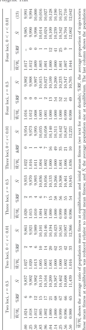
First, this informs us thatNˆ ⱖK⫽ ␬(␳ ⫺1) if and only ifVA⫽ 0 or

fⱖ 1

2(␳ ⫺1) (14)

because the denominator of the last term in (13) is always positive (recall that we haveVAⱕ1⁄8,V␣ⱖ1⁄2, and

Vsⱖ1⁄8if␪ ⫽1⁄2). Table 4 shows that (14) predicts the

valuefat whichNˆ _⫽Knearly correctly (althoughg⫽ ␪

is assumed in its derivation), namelyf ⫽ 0.5 if␳ ⫽ 2. Second, numerical evaluation of (13) shows that it in-deed provides a very accurate approximation of the numerically observed averageNˆ (compare the last two columns in Table 4). This is also the case for all other parameter combinations of Table 4, as well as for many others (e.g., for other values of ␳ and ␬; results not shown).

Differentiation of (13) with respect to V␣shows that

TABLE 4 Properties of equilibrium m ean fi tness and population size Two loci, r ⫽ 0.5 Two loci, 0 ⬍ r ⬍ 0.01 Three loci, r ⫽ 0.5 Three loci, 0 ⬍ r ⬍ 0.01 Four loci, r ⫽ 0.5 Four loci, 0 ⬍ r ⬍ 0.01 f Wˆ /W 0 %RF Nˆ Wˆ /W 0 %RF Nˆ Wˆ /W 0 %RF Nˆ Wˆ /W 0 &RF Nˆ Wˆ /W 0 %RF Nˆ Wˆ /W 0 %RF Nˆ (13) 0.00 1.024 6 9,837 1.027 2 9 ,861 1.020 2 9,953 1.022 0 9,954 1.016 0 9,982 1.017 – 9,985 9,991 0.25 1.018 9 9,902 1.020 4 9 ,921 1.015 3 9,970 1.016 1 9,973 1.012 0 9,988 1.012 0 9 ,990 9,994 0.50 1.012 1 2 9 ,982 1.013 6 9 ,989 1.010 4 9,993 1.011 1 9,995 1.008 0 9,997 1.009 0 9 ,998 10,000 0.83 1.005 1 5 1 0,110 1.005 10 10,101 1.004 6 10,036 1.004 4 10,035 1 .003 1 10,015 1.003 1 1 0,014 10,016 0.96 1.002 1 7 1 0,164 1.003 14 10,146 1.002 7 10,056 1.002 7 10,058 1 .001 2 10,027 1.001 1 1 0,024 10,027 1.04 1.000 2 1 1 0,209 1.001 20 10,194 1.000 1 5 10,133 1.000 16 10,140 1 .000 1 3 10,109 1.000 12 10,109 10,128 1.14 1.000 6 8 1 0,387 1.000 62 10,423 1.000 5 8 10,266 1.000 49 10,311 1 .000 5 4 10,200 1.000 41 10,239 10,190 1.25 0.999 6 7 1 0,462 1.000 53 10,581 0.999 5 6 10,308 1.001 35 10,442 1 .000 5 2 10,233 1.001 25 10,342 10,237 1.56 0.996 6 6 1 0,688 1.002 42 10,997 0.998 5 5 10,461 1.006 21 10,847 0 .999 5 1 10,347 1.007 9 1 0,704 10,710 2.50 0.988 6 5 1 1,439 1.016 33 12,366 0.996 5 4 10,945 1.036 10 12,221 0 .998 4 9 10,705 1.044 1 1 2,062 12,042 Wˆ /W 0 shows the average ratio of population m ean fi tness at equilibrium a nd initial mean fi tness (see text for m ore details); %RF, the average p roportion o f trajectories whose m ean fi tness at equilibrium w as reduced relative to initial mean fi tness; and Nˆ , the average population size at equilibrium. The last column shows the population size calculated from the approximation (13) using the observed genetic variance for four tightly linked loci. The parameters ␬⫽ 10,000, ␳⫽ 2, Vs ⫽ 1.25, ␪⫽ 0.5 are as in Tables 1 a nd 2.

which is only slightly larger than one. Hence, Nˆ in- A potentially important conclusion resulting from Equations 10, 11, and 15 is that for small growth rates creases with f unless ␳ is very small. Table 4 confirms

this. This is in accordance withAsmussen(1983), who ␳, much largerf, hence stronger competition, is needed to induce a qualitative change in the equilibrium struc-showed for rather general one-locus models of FDS that

the population size at a stable interior equilibrium can ture becauseφD⬎φS⬎ ␽ˆ ⬇ (␳ ⫺1)⫺1. This is not

im-mediately obvious for models based on the Lotka-Volt-exceed the carrying capacity if intraspecific competition

erra functional form (e.g.,Slatkin1979), in which the between like genotypes is stronger than that between

location of this region would depend on ␴2

k/V␣, where unlike genotypes. In Slatkin’s (1979)

quantitative-␴2

k is the width of the available resources. However, genetic model of Lande’s kind, the population size at

since Equation 19 ofBu¨ rger(2002b) informs us that the equilibrium with nonzero genetic variance is

pro-␴2

kis proportional toVswith proportionality constant␳␬/

portional to 1/

√

N⫺1, the models indeed lead to equivalent predictions. Equation 13 predicts that the equilibrium population

These multilocus results confirm and generalize the size is always proportional to␬, and this has been verified

conclusion of Bu¨ rger (2002a,b) that, compared with numerically (results not shown). Another important

pure stabilizing selection, FD leads to a quantitative, but point is (Table 4) that for a wide range of valuesf, the

not to a qualitative change, in the equilibrium proper-equilibrium population size deviates from Kby only a

ties of genetic variation as long as f⬍ ␽ˆ ⬇(␳ ⫺1)⫺1_.

few percent [cf. (13) and recall that on average VA is

Only larger f induces a qualitative change. Notably, very small]. Therefore, we have

the critical value at which this occurs is independent of the number of loci.

␽ˆ _{⫽ ␳␬}

Nˆ ⫺ 1⬇

1

␳ ⫺1, (15) The asymmetric case:Now we turn to the asymmetric case and explore the consequences of a shifted opti-which equals 1 if and only if␳ ⫽2. Table 4 also shows that _{mum. Even in the absence of FD,i.e., for pure stabilizing} the deviation ofNˆ fromKdecreases with an increasing _{selection, very little work on the asymmetric case has} number of loci. This is confirmed by (13) because (un- _{been done and no simple, general results are available} less linkage disequilibrium is extremely high) in our _{(Hastings andHom 1990;Gavrilets andHastings} model the averageVAdecreases with increasing number _{1993; Bu¨ rger2000, pp. 213–216). Our numerical}

re-of loci since the average effect re-of a locus decreases in _{sults are based on the assumption of free recombination}

proportion to 1/(2n). _{and that the position of the optimum is at ␪ ⫽ 0.75.}

Numerical iterations for various ecological parameter _{The main findings are summarized in Figure 2 and}

sets in which ␬ has been changed by a factor of 10 _{Tables 5 and 3, which compare the asymmetric case}

show that the only statistically significant effect on the _{with the corresponding symmetric case from Figure 1} properties of the system is that the carrying capacity and, _{and Table 1. Figure 2 clearly demonstrates the existence} hence, the equilibrium population size are changed by _{of a transitory region and shows that its lower bound is} the corresponding factor. Similarly, different values of _{nearly unaffected by the shift in the optimum, as}

pre-␳ induce exactly the transformation indicated by (10), _{dicted by our theoretical estimate (10) (for ␪ ⫽ 0.75,} (11), and (13), but have no statistically significant effect _{we obtainφS ⫽1.06␽ˆ instead of the previous 1.03␽ˆ , and} on the relative genetic variance, the number of equilib- _{␽ˆ is nearly identical in both cases). However, although} ria maintained, or their degree of polymorphism (re- _{there is a distinctive increase of both the relative genetic} sults not shown). For␳ ⬎3, the dynamics ofNbecome _{variance and the polymorphism in a small range of} complicated and were not studied in detail. However, _{valuesf, there is no clear upper bound of the transitory} in the few runs performed the dynamics of gamete fre- _{region. Instead, both quantities increase very slowly} un-quencies seemed to be nearly unaffected by the fluctua- _{tilf⫽2.5 is reached. For the given strength of} stabiliz-tions of the population size. A similar observation was ing selection (Vs ⫽ 1.25), this is the largest possible

reported byClarkeandBeaumont(1992). value in this model and attained ifV␣⫽0.5.

If density dependence is ignored and the population For weak or moderate FD (f ⬍ 1), the degree of size is assumed constant and equal toK, then up to a polymorphism is unaffected by the change in␪ (com-scale transformation of f by the factor (␳ ⫺1)␽ˆ , the pare Table 5 with Table 1, and see Table 3) and, except same results as for a changing population size are ob- for two loci, asymmetry leads only to a slight loss of tained. For instance, for a fixed population size of genetic variance. For five loci, the difference nearly van-10,000, the relative genetic variance and the polymor- ishes. If FD dominates (f ⬎ 1.1), then a shifted opti-phism at some valuefare about the same as those for mum leads to substantially reduced genetic variance variableN at the value (␳ ⫺1)␽ˆf(results not shown). and polymorphism relative to a symmetric one. Under Thus, for fixed population size, the critical values φS the strongest possible FD in our model, the relative

and φD are somewhat larger than those under density genetic variance and the average amount of

polymor-dependence because, by (14),Nˆ ⬎Kiff⬎1_⁄

2(␳ ⫺1)⫺1. phism still are diminished byⵑ20% relative to the

were also obtained for an optimum at the upper bound-ary of phenotypic values,i.e., for␪ ⫽1. Then the trait is under pure directional selection if FD is absent. We found that for free recombination, four loci,Vs⫽1.25,

and the strongest possible FD,i.e.,f⫽2.5, the relative genetic variance is only 0.4, the average polymorphism is 2.0, and four-locus polymorphisms have a frequency of⬍0.02. For weak FD (f⫽0.83), no polymorphism at all is maintained. This is consistent with the finding of LoeschckeandChristiansen(1984) that for a single locus with multiple alleles, even under strong FD, no variation is maintained if the trait is under directional selection.

We also computed standard deviations of our quanti-ties of interest. For three, four, and five loci, the stan-dard deviation of the relative genetic variance is nearly twice the mean in the absence of FD and decreases to a value close to the mean as f increases to φS. This

holds for both recombination scenarios and for␪ ⫽0.5 and␪ ⫽0.75. Hence, genetic variation between genetic systems varies greatly for weak to moderate FD. Under free recombination, the standard deviation decreases further in absolute terms as f increases and is always

⬍2% of the mean if f ⬎ φD. Hence, the genetic

vari-ance maintained under strong FD is nearly independent of the locus effects. For tight linkage, the standard de-viation of the variance is between 15 and 20% of the mean iff⬎ φD; thus in absolute terms it increases for

Figure2.—Relative genetic variance (a) and polymorphism _largef. (b) as a function off⫽Vs/V␣forn⫽2, 3, 4, and 5 loci in

the case of free recombination. The symmetric case (␪ ⫽

0.5) is compared with the asymmetric case (␪ ⫽0.75). The _{DISRUPTIVEVS.STABILIZING SELECTION} parametersVs, ␳, and ␬are as in Figure 1 and V␣is varied;

hence the data for␪ ⫽0.5 are those of Figure 1, except that Analysis of the conditions under which FDS induces data for some valuesfare omitted here. Instead, the range of _{disruptive selection on a trait is of importance because} valuesfis extended here up to the maximum possiblef⫽2.5 _{disruptive selection is a prerequisite for sympatric} speci-in this model to demonstrate the effects of an asymmetric

ation if it is to be induced by competition. The fitness optimum more clearly. The bars between a and b indicate

function in our model, (4), is a polynomial of degree which type of selection was observed in the asymmetric case,

␪ ⫽0.75 (cf. Figure 1 for␪ ⫽0.5). 4 ing, and we classified its shape as傽-shaped (concave with a local maximum), resulting in stabilizing selection, 傼-shaped (convex with a local minimum), resulting in polymorphic. Actually, the more loci there are, the disruptive selection, or else, which we call complicated lower the fraction of fully polymorphic equilibria. The selection. The fitness function was calculated at each stable relative genetic variance depends only very weakly on equilibrium and classified according to one of the three the number of loci. The deviation of the mean from categories. For a symmetric optimum (␪ ⫽0.5), a fitness the optimum is about as small as in the symmetric case function classified as complicated is M-shaped in all

(results not shown). cases examined; i.e., there are two local optima (not

Thus, for weak or moderate FD (f ⱕ φS), free re- at the extreme genotypic values) separated by a local

combination, and three or more loci, a shift in the minimum. The shape of theM, however, can be rather optimum of small or moderate size (i.e., 0.25 ⱕ ␪ ⱕ variable because the minimum can be very shallow or 0.75 so that␪is closer to the middle of the phenotypic very deep, and the fitness of the extreme genotypic range than to its boundaries) has only a minor effect values can be very low or just slightly lower than the on the amount and structure of the genetic variation maximum. TheMis asymmetric ifg⬆␪.For an asym-at equilibrium. For two loci, the effect is much larger metric optimum or at unstable equilibria in the symmet-because a shifted optimum destroys the inherent sym- ric case, other shapes may occur, such as monotone metries of the two-locus model that maintain much decreasing or increasing fitness, or one local maximum more relative genetic variance than that in models with and one local minimum.

TABLE 5

Equilibrium structure forn⫽2, 3, and 4 loci, free recombination, and an asymmetric optimum (␪⫽0.75)

Two loci Three loci Four loci

Polymorphism Polymorphism Polymorphism

f No. (E) 0 1 2 No. (E) 0 1 2 3 No. (E) 0 1 2 3 4

0.00 1.5⫾0.5 0.50 0.50 0 2.4⫾0.8 0.52 0.48 0 0 2.8⫾1.0 0.62 0.38 0 0 0

0.25 1.5⫾0.5 0.35 0.65 0 2.5⫾0.8 0.39 0.61 0 0 2.9⫾1.1 0.48 0.52 0 0 0

0.50 1.5⫾0.5 0.25 0.75 0 2.6⫾0.9 0.26 0.74 0 0 3.0⫾1.1 0.32 0.68 0 0 0

0.83 1.6⫾0.5 0.10 0.90 0 2.7⫾0.9 0.09 0.91 0 0 3.3⫾1.2 0.11 0.89 0 0 0

0.96 1.7⫾0.5 0.03 0.97 0 3.0⫾0.9 0.02 0.98 0 0 3.6⫾1.2 0.03 0.97 0 0 0

1.04 1.9⫾0.3 0 1 0 2.2⫾0.5 0 0.40 0.60 0 2.7⫾0.7 0 0.20 0.53 0.27 0

1.14 1 0 0.71 0.29 1 0 0.22 0.50 0.29 1 0 0.06 0.29 0.44 0.21

1.25 1 0 0.49 0.51 1 0 0.13 0.48 0.39 1 0 0.03 0.23 0.47 0.26

1.56 1 0 0.38 0.62 1 0 0.09 0.46 0.45 1 0 0.02 0.19 0.49 0.31

2.50 1 0 0.26 0.74 1 0 0.05 0.40 0.55 1 0 0.01 0.14 0.48 0.37

See Table 1 for definition of parameters.

by a quadratic polynomial through regression. There- side of (17) coincides withφD(11). Therefore, disruptive

selection occurs for all possible genetic systems in this fore, we also approximated our fitness function by a

quadratic polynomial and classified it as stabilizing selec- model iff⬎ φD. These results suggest that in the

sym-metric case, disruptive selection should be almost always tion if it was concave (curved downward) and as

disrup-tive otherwise. detectable if FD is strong enough to maintain a unique

fully polymorphic equilibrium. In Figures 1 and 2, the horizontal bars below the top

section display the dependence of the shape of the For the asymmetric optimum, the region with compli-cated selection is substantially extended and much fitness function on f. Except for the region in which

selection is complicated, the same type of selection oc- stronger FD is needed to produce disruptive selection (Figure 2). This is also predicted by (17), which gives curs at all equilibria and for all genetic parameter

com-binations. The coincidence between the type of selec- a critical value offbetween 1.7 and 1.9 if VA⫽ 1⁄8and

the numerically obtained Nˆ’s (in this region between tion acting and the properties of genetic variation

maintained at equilibrium is remarkable. The figures 10,300 and 10,800) are plugged in. In the transitory region (and only there), the fitness function is often clearly show that complicated selection occurs in the

transitory region,i.e., if φS⬍ f⬍φD. Under the assump- not only complicated, but also very flat near

equilib-rium, thus leading to extremely slow convergence (cf.

tion that the mean coincides with the optimum, g⫽ ␪

(as is satisfied to a close approximation for the vast the statistical approach). majority of parameter combinations if more than two

loci contribute to the trait—the more loci, the better

EVOLUTION OF MEAN FITNESS the approximation), it is straightforward to show that

W(g) is傽-shaped if and only if

For two loci and by ignoring density dependence, it was shown (Bu¨ rger 2002b) that under moderate or strong

f⬍ ␽ˆ ⫹ VA

2V␣. (16) FD, the dynamics in this model may be highly nonadaptive;

i.e., mean fitness may often decrease and critical points Since by (10), monomorphic equilibria exist iff⬍ φS⫽ of the fitness surface bear little relevant information

␽ˆ _{⫹1/(8V␣), (16) is satisfied for all possible genetic}

about the dynamics or equilibrium properties of the

parameter combinations if and only iff⬍ ␽ˆ . _{model. However, even if a stable polymorphism}

coin-Another straightforward calculation shows that if _{cides with a critical point of the fitness surface, methods}

g⫽ ␪ ⱖ1_⁄

2(as is approximately the case in our numeri- relying on the invasion analysis of a rare mutant in a

cal results) disruptive selection occurs if and only if the _{monomorphic population may be insufficient for} deriv-derivative ofW(g) atg⫽0 is positive. This is the case _{ing the correct evolutionary properties of this}

equilib-if and only equilib-if _{rium (Christiansen1991).}

For the present multilocus model we investigated

f⬎ ␽ˆ ⫹VA⫹ 2␪

2

2V␣ ⫽ ␽

ˆ

冢

2Vs

冣

⫺1

. (17) such and related issues using our statistical approach. For every trajectory, we calculated the ratioWˆ /W0of the

mean fitness at equilibrium (which, of course, is one) If␪ ⫽1_⁄

2andVA⫽1⁄8, which is the largest possible value

1000 genetic parameter sets pertaining to a given eco-logical parameter combination. Because initial points are randomly chosen, the average ratioWˆ /W0provides

a measure for the net change of population mean fitness during evolution. We also calculated the percentage of trajectories, %RF, for which mean fitness at equilibrium was lower than that initially. Some of these results are summarized in Table 4.

A number of noteworthy features are observed. As f

increases from zero, the average ratioWˆ /W0decreases

from a value⬎1 to 1.000 asfreachesⵑ1.0 (⬇φS). In

parallel, the proportion of trajectories for which fitness is reduced at equilibrium increases from nearly zero (except for two loci, when this proportion is a few per-cent) to 10% or more. This percentage reaches a maxi-mum of 40% or more in the transitory region and de-clines asfincreases beyondφD. For free recombination

this decline is very slow, but for tightly linked loci it is rapid; the more loci, the more rapid the decline.

Wˆ /W0decreases slightly below one forf⬎φDif

recombi-nation is free, but increases quite substantially if linkage is tight. Therefore, under moderate or strong FD (f⬎

φS) the dynamics are “on average” nonadaptive if the

loci are unlinked. However, if the loci are tightly linked and FD is very strong, then mean fitness decreases only with low probability and, on average, increases substan-tially above that of randomly chosen initial distributions.

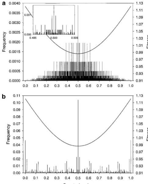
Figure 3.—Frequencies of genotypic values and fitness As we see by way of example in the next section, this is

function at equilibrium for four loci. The locus effects are because with tightly linked loci, the phenotypic distribu- _{␥1 ⫽ 0.036, ␥2 ⫽ 0.250, ␥3 ⫽ 0.191, and ␥4 ⫽ 0.023; the} tion shows signs of clustering at its extreme phenotypic _{ecological parameters areVs⫽1.25,V␣⫽0.5,␳ ⫽2, and␬ ⫽} 10,000. Hence there is a unique, globally stable equilibrium values.

with all allele frequencies equal to1_⁄

2. Only the linkage

disequi-libria depend on the genetic details. The 傼-shaped curve depicts the fitness function at this equilibrium. Its scale is PHENOTYPIC DISTRIBUTIONS AT EQUILIBRIUM

given on the right-hand side. (a) Freely recombining loci. Most ecological modeling focusing on the evolution- _{(b) Recombination rates between adjacent loci are randomly} chosen between 0 and 0.01 and are 0.0089, 0.0037, and 0.0041 ary consequences of FDS has relied on assumptions

in this case. There are as many vertical bars (34⫽_{81 genotypic}

about the distribution of genotypic or phenotypic

val-values) in b as in a, but many are invisible because their height ues. Models using the quantitative genetics approach

is so small. assume that phenotypic values are normally distributed

(and do not change shape), whereas models resorting

to game theory or adaptive dynamics consider the fate of have much higher frequencies. In particular, with tight linkage the extreme genotypic values occur with high fre-single mutants in otherwise monomorphic populations.

Figures 3 and 4 show how distributions of genotypic quency. Because of random mating, however, the central genotypic value is always the most frequent one.

values look in four- and eight-locus models if FD is

strong,i.e., such that a unique, fully polymorphic, stable We end with a little lesson on the central limit theo-rem. Despite its fractal appearance, the distribution for equilibrium exists. They display seemingly fractal

fea-tures;i.e., typically the frequencies of neighboring geno- eight loci and free recombination in Figure 4a is nearly normal. Figure 5 displays its cumulative density function typic values are radically different. Only a few runs with

eight loci were performed with the sole purpose of dem- together with that of a normal distribution with the same mean and variance. Also the cumulative density onstrating the equilibrium distribution.

Figure 3, a and b, as well as Figure 4, a and b, differ functions of the other distributions displayed in Figures 3 and 4 are shown. The distribution resulting from eight only because of different assumptions on the

recombi-nation rate; all other parameters, including the allelic tightly linked loci and those from four loci (linked or not) are markedly nonnormal. That the eight-locus dis-effects, are the same. Comparison of these pairs of

fig-ures shows that with tight linkage a much larger fraction tribution with free recombination is nearly normal is a consequence of the central limit theorem together with of genotypic values has very low frequency compared with