ABSTRACT
LEE, HEE WON. Network Emulation with Adaptive Time Dilation. (Under the direction of Mihail L. Sichitiu and David Thuente.)
© Copyright 2015 by Hee Won Lee
Network Emulation with Adaptive Time Dilation
by Hee Won Lee
A dissertation submitted to the Graduate Faculty of North Carolina State University
in partial fulfillment of the requirements for the Degree of
Doctor of Philosophy
Computer Science
Raleigh, North Carolina
2015
APPROVED BY:
Rudra Dutta Xuxian Jiang
Mihail L. Sichitiu
Co-chair of Advisory Committee
David Thuente
DEDICATION
BIOGRAPHY
ACKNOWLEDGEMENTS
TABLE OF CONTENTS
LIST OF TABLES . . . vii
LIST OF FIGURES . . . .viii
Chapter 1 Introduction . . . 1
1.1 Overview . . . 2
1.2 Node Emulation . . . 4
1.3 Link Emulation . . . 4
1.4 Time Dilation . . . 5
Chapter 2 Related work . . . 7
2.1 Real-time Network Emulation . . . 7
2.2 Large Testbeds . . . 8
2.3 Network Simulation . . . 8
2.4 Hybrid Simulation and Emulation: . . . 9
Chapter 3 High-performance Emulation of Heterogeneous Systems using Adap-tive Time Dilation . . . 10
3.1 Emulating Heterogeneous Systems . . . 11
3.1.1 Full Virtualization . . . 11
3.1.2 Abstraction Layer of Time Control . . . 12
3.2 Adaptive Time Dilation . . . 13
3.2.1 Slice-based Time Dilation . . . 14
3.2.2 Adaptation of Dynamic Time Dilation to System Loads . . . 15
3.3 System Architecture and Implementation . . . 18
3.3.1 Synchronization . . . 18
3.3.2 Synchronization Agent . . . 19
3.3.3 System Tuning . . . 20
3.4 Performance Evaluation . . . 26
3.4.1 Experimental Setup . . . 26
3.4.2 Emulation Accuracy . . . 27
3.4.3 Heterogeneity . . . 28
3.4.4 Scalability . . . 31
3.4.5 Real-world Application: VLC media player . . . 32
3.5 Summary . . . 33
Chapter 4 Network Link Emulation with Adaptive Time Dilation . . . 34
4.1 Approach . . . 35
4.1.1 Virtual Link Design . . . 36
4.1.2 TDF Control . . . 38
4.2 System Implementation . . . 39
4.2.2 Virtual Link Implementation . . . 39
4.2.3 System Load Control . . . 43
4.3 Performance Evaluation . . . 43
4.3.1 System Parameters . . . 44
4.3.2 Delay Control . . . 45
4.3.3 Emulated Delay . . . 47
4.3.4 Virtual Link Under Traffic Loads . . . 50
4.3.5 High Throughput and Low Latency . . . 53
4.3.6 Real-world Application . . . 54
4.3.7 System Overhead . . . 57
4.4 Summary . . . 57
Chapter 5 Integrated Simulation and Emulation Using Adaptive Time Dilation 58 5.1 Approach . . . 59
5.1.1 The Effects of Time Dilation on Simulation . . . 60
5.1.2 The Effects of Time Dilation on Emulation . . . 63
5.1.3 Virtual Time . . . 63
5.1.4 Adaptive Time Dilation . . . 64
5.2 System Implementation . . . 65
5.2.1 System Architecture . . . 65
5.2.2 Virtual Time Implementation . . . 66
5.2.3 TDF for System Load Control . . . 67
5.3 Performance Evaluation . . . 67
5.3.1 Experimental Setup . . . 68
5.3.2 TDF Controller Tuning . . . 68
5.3.3 Evaluation Topology . . . 69
5.3.4 Outgoing Packet Delay . . . 70
5.3.5 Evaluation of Adaptive Time Dilation . . . 74
5.4 Summary . . . 78
Chapter 6 Conclusion and Future Work . . . 79
6.1 Conclusion . . . 79
6.2 Future Work . . . 80
LIST OF TABLES
Table 3.1 Each OS’s clock source changes to HPET or PIT for virtual time. . . 13
Table 3.2 Software packages used in our emulation system. . . 26
Table 3.3 Specification of sample video files . . . 33
LIST OF FIGURES
Figure 1.1 Overview of proposed network emulation with the mapping of the virtual
elements to physical hosts . . . 3
Figure 3.1 Illustration of slice-based time dilation . . . 14
Figure 3.2 TDF controller . . . 16
Figure 3.3 The synchronization agent on each PH determines a current TDF and dis-seminates it to all VHs on that PH. . . 19
Figure 3.4 Activity diagram of synchronization agent . . . 20
Figure 3.10 A streaming service topology is created for evaluating heterogeneity. . . 28
Figure 3.13 A virtual network topology for evaluating scalability. . . 31
Figure 3.15 (a) A virtual network topology for evaluating the VLC media player that runs on our emulation system (b) Higher video bitrates imply larger TDF. 32 Figure 4.1 Overview of proposed network emulation with the possible mapping of the virtual elements to physical hosts . . . 36
Figure 4.2 Delay components of a virtual link . . . 37
Figure 4.3 TDF control mechanism . . . 38
Figure 4.4 A sample virtual network in (a) can be emulated by our system, as depicted in (b). . . 40
Figure 4.5 Virtual link implementation . . . 41
Figure 4.6 After measuring RT TvlinkV |T DF=1 and RT TbypassR , we compute delayV HsR by (4.11). . . 44
Figure 5.1 (a) Example topology with an integrated emulation and simulation system with the simulator sending one packet to the emulator. (b) If the simulator is overloaded, outgoing packets can be delayed with respect to their original scheduled times. . . 59
Figure 5.2 Overview of the proposed approach with (a) an example of a real world topology and (b) a possible mapping of the virtual elements to physical hosts 60 Figure 5.3 The effect of reduction in outgoing packet delay by time dilation. (a) The simulator transforms a live packet into simulation events, processes the events, and creates an outgoing packet. (b) Real-time scheduler running in real time (TDF=1) introduces outgoing packet delay. (c) Time dilation, where virtual time passes at half the rate of real time (TDF=2), can reduce outgoing packet delay. (d) An even larger TDF=4 can completely eliminate outgoing packet delay. . . 61
Figure 5.4 Synchronization of virtual elements . . . 63
Figure 5.5 Virtual time control mechanism using TDF to control the system load . . . 64
Chapter 1
Introduction
Distributed systems rely on the collaboration of a large number of nodes. Due to complex interactions, it is difficult to evaluate their performance without building prototypes. Diverse techniques, such as theoretical analysis, simulation, testbed implementation and emulation, have been used for evaluating their performance.
Theoretical analysis provides elegant solutions for relatively simple systems [36, 59]. As long as underlying assumptions are reasonably satisfied, the results of the analysis often offer exceptional insights that cannot be obtained through any other method. However, theoreti-cal analysis frequently requires simplifying assumptions, which may make meaningful analysis extremely difficult [36].
Simulation allows for reasonably convenient testing, with relatively complex scenarios, while avoiding overly simplistic assumptions. However, the accuracy of the simulation results is heav-ily dependent on the accuracy of the models employed in the simulation. Subtle changes of parameter values in a simulation model may render many simulation results invalid. Further-more, the many of simulation experiments are not easily repeatable [70], and the results of each simulation package for a common scenario can be very different from one another or from real testbed results [65].
Testbed measurements offer the most accurate and realistic results, but actual physical systems are needed. This considerably restricts the range of network topologies and protocols that can be tested. Moreover, testbeds often require large expenditure of time and money to set up and maintain.
to emulate multiple virtual hosts (VHs). An unmodified OS can run on a hypervisor, and unmodified applications, in turn, can be executed on the unmodified OS. Emulation based on VHs is useful to make efficient use of computing resources because VHs can be deployed to maximize the overall utilization of physical resources. However, the results of emulation are compromised if the loads on the PHs exceed the PHs’ resources.
In this dissertation we propose to use emulation as a flexible, yet realistic way, to evaluate the performance of real networking systems. In the proposed approach, we emulate virtual network nodes such as routers, switches, hosts, and servers and connect them with virtual links in a virtual network. In addition, it is possible to have wide area networks (WANs) participate as an element in a virtual network [4, 16]. Simulators can also be used to introduce elements not available for emulation into the virtual network. Real networking protocols work in all emulated elements and real packets will be exchanged between the elements just as in a real network. To allow the networks to scale, we use a distributed implementation, where N host computers emulate M virtual elements and M can be much larger than N.
The main advantage of the proposed emulator is its realism, since each node runs unmodified operating systems (OSs) and protocol implementations. The second advantage is its flexibility, as changes in the network topology can be made as simple as in network simulators. Finally, the proposed emulator uses commodity hardware, thus allowing a straightforward and cost-effective dissemination of the system to the larger community.
An important characteristic of our approach is that our emulation system can be used to test heterogeneous systems consisting of distributed nodes running different OSs. With our em-ulation system, it is possible to emulate Internet applications and services, which are supported by diverse OSs such as Windows, FreeBSD, Linux, Cisco IOS, Juniper Junos, etc. To emulate heterogeneous OSs, we use QEMU-KVM [25, 11] that supports full virtualization. Our solu-tion allows multiple VHs to be created on the same PH with each VH capable of generating heavy network traffic; the adaptive time dilation employed in our solution allows for an accurate emulation of the virtual network without performance degradation.
1.1
Overview
Network emulation is a technique that combines real elements of a deployed networked appli-cation such as end hosts and protocol implementations with synthetic, simulated, or abstracted elements such as network links, intermediate nodes and background traffic [53]. An emulated network is a collection of emulated nodes and emulated links [40].
can be built with limited physical resources. Conversely, if the system emulated requires very few resources, it can be emulated faster than real time.
For the network emulation system, each network element in the desired topology will be instantiated as a virtual element that runs on a PH. For scalability, multiple PHs can be used for mapping the virtual network elements to host machines. Once all elements are ready to start, the emulation will proceed at a variable time rate in a synchronized manner.
Server
Routers
Windows clients
Linux clients
FreeBSD clients
...
... ...
(a) Real-world topology
Virtual Server PH1
...
Virtual Router
Virtual Router
Virtual Windows
Virtual Linux
Virtual FreeBSD Virtual
Router
Virtual Router
... ...
PH2
PH3 PH4 PH5
Virtual Link
Synchronized Virtual Time
(b) Emulation topology
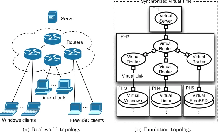
Figure 1.1: Overview of proposed network emulation with the mapping of the virtual elements to physical hosts
Fig. 1.1(a) depicts a sample network with Windows/Linux/FreeBSD clients connected to a server through routers. Fig. 1.1(b) shows a possible mapping of the elements in the real-world topology into virtual elements emulated on five physical machines. The clients, server, and routers may be emulated via a virtualizing technology such as QEMU-KVM [25, 11], Xen [31], and VMWare [30].
1.2
Node Emulation
Hosts and routers are emulated as network nodes in our system. Emulated hosts are referred to as virtual hosts (VHs). Unmodified OSs run on hypervisors, and unmodified applications or protocol implementations, in turn, can be executed on the unmodified OSs.
There are several hypervisors that can create and run virtual machines (VMs), each running a separate OS instance. QEMU-KVM [25, 11], Xen [31], and VirtualBox [29] are popular and free hypervisors, while VMWare [30] is a commercial product.
Many academic research efforts have been based on Xen [31], but the QEMU-KVM hyper-visor is recommended as the optimal choice for high performance computing environments [77]. Furthermore, QEMU-KVM runs each guest OS as a separate process in a PH, so established OS mechanisms such as shared memory and interprocess communications can be used to add new features to the hypervisor. QEMU-KVM can perform at near native speed with the KVM kernel component addition that provides a full virtualization solution. Hence, we choose QEMU-KVM to create VHs in our emulation system.
For emulating routers, we use Olive [20], which allows Junos [10] to run on a VM provided by the QEMU-KVM hypervisor.
1.3
Link Emulation
From the perspective of a host OS, each VH is a process, and the VHs communicate with one another via virtual links, which are implemented through inter-process communications [73] or using the Universal TUN/TAP device driver [28].
TUN/TAP provides packet reception and transmission for user space programs. Instead of receiving or transmiting packets from a physical media, a TUN/TAP device driver receives or transmits them from a process in the user space.
QEMU-KVM provides several methods for setting up virtual links for its VHs. As an inter-process communication method, QEMU-KVM can connect multiple guest systems on a VLAN, which is a network switch running in the context of a QEMU process, using TCP or UDP sockets. Another method is to use TAP interfaces to provide full networking capability [26]. Virtual links between VHs are built such that TAP interfaces on VHs connect to each other through an Ethernet bridge [13] provided by the Linux kernel. Furthermore, an Ethernet bridge enables a TAP interface of the VH to connect to the PH’s interface. This allows a VH to connect to another VH on a different PH.
delay, bounded-size queue, packet losses, multipath, etc. EmuNET has been designed to test protocols under a variety of conditions, such as bit rate limitations, network delay and jitter, different queuing schemes, etc [58]. NetEm [54, 16] emulates variable delays, packet losses, duplication and reordering. Tc [12] can classify traffic and limit bandwidth. We use Tc [12] and NetEm [54, 16] to reproduce the effects of designated rates and delays on packets passing through a virtual link in our system.
1.4
Time Dilation
Using VHs in network emulation makes it possible for time to pass at a rate different from physical time. Thetime dilation is a technique to uniformly slow the passage of time from the perspective of an operating system by a specified factor [52]. If only one second passes in VHs for everyx seconds of wall clock time, physical resources appearxtimes faster. This is particularly important for network emulation, since time dilation does not change a packet arrival rate. Therefore, time dilation enables empirical evaluation at network speeds and capacities that are not currently available from production hardware.
DieCast [51] scales CPU cycles, network communication characteristics, and disk I/O and thus providing the illusion that each VM matches its original machine in terms of available computing resources and communication behavior to remote service nodes. The behavior of DieCast therefore matches that of the original service at a fraction of actual physical resources. However, the main limitation of DieCast is that the scaling factor cannot be changed during run time.
The Distributed Open Network Emulator (dONE) employs a temporal model called rela-tivistic time, which is conceptually the same technique as time dilation. dONE reconciles the real-time nature of direct code execution with the event driven nature of simulation models [35]. In addition, dONE creates VHs using a composition framework called Weaves, which provides the ability to emulate multiple instances of an application or protocol stack inside a single OS process [67]. The design goal of dONE is to enhance scalability in building hybrid emula-tion/simulation environment and to do this using relativistic time on the Weaves Framework.
with the network simulation [75]. Time in VHs proceeds only when the synchronization com-ponent allocates the next time slice. Otherwise, time in VHs remains stalled. The approach in SliceTime [76] is to alternately suspend and resume the entire system in order to connect VMs to discrete event simulations [62] that may lag behind in time under heavy system loads [75].
The approaches in [75, 76, 52, 51] are static in that the relative ratio between real and virtual time is fixed for the life of the VMs. Compared to a constant clock rate that results in suboptimal experiment runtime, network emulation using adaptive virtual time [45] dynamically adjusts the clock rate to system loads. The work in [45] uses the concept of epoch-based virtual time [48] where the experiment is divided in epochs, each of which has a constant time dilation factor (TDF). The TDF adaptation process is based on threshold-based adaptive sampling of system loads [45]. NETplace [46] and NETbalance [47] also use epoch-based virtual time for implementing a dynamic time dilation.
Chapter 2
Related work
2.1
Real-time Network Emulation
CORE (Common Open Research Emulator) deploys a real-time network emulator with a hybrid approach, using a network stack of routers or hosts through virtualization and simulating the links that connect them together [33]. CORE uses the FreeBSD network stack virtualization provided by the VirtNet [27] project. The lightweight virtualization, where only part of the OS is made virtual, allows CORE to scale to over a hundred virtual machines running on a single emulation server. For wireless emulation, CORE focuses on realistic emulation of layer 3 and above, and does not model layer 1 and 2 of a wireless protocol such as 802.11.
Wireless channel emulators use hardware to simulate wireless channel propagation in real time. The reason for using hardware is that emulation must be fast to operate in real time, flexible to capture many different environments, and accurate to ensure that the radio signals are not distorted. There are a number of such wireless emulators [71] [57], including the FPGA-based Channel Simulator [37].
RAMON, a Rapid-Mobility Network emulator, is a software/hardware emulator that mimics realistic characteristics of wireless networks [55]. RAMON allows the ns-2 simulator to interact with actual hardware components including access points (APs), attenuators, laptops, and smart phones, while emulating mobility in wireless networks.
mainly for testing the protocols at layer 3 and above.
2.2
Large Testbeds
Several large testbeds, which partially use emulation techniques or significantly depend on them, have been developed. PlanetLab is a geographically distributed overlay network designed to support the deployment and evaluation of planetary-scale network services[34]. PlanetLab enables multiple services to run concurrently, each in its own slice of PlanetLab [24, 41]. Em-ulab [5] provides researchers with integrated access to emulated PC nodes, an 802.11 a/b/g testbed, and universal software defined radios (USRP devices). Additionally, Emulab can be expanded into PlanetLab testbeds, enabling live Internet experimentation. GENI [6] is a NSF initiative that supports at-scale experimentation on shared and heterogeneous infrastructure. GENI provides researchers across the country with collaborative environments on which new network architectures and their implementations can be tested. DETERlab [3] is a testbed designed to support research and development on next-generation cyber security technologies. DETERlab uses the Emulab cluster testbed software that allows for controlling and managing a pool of PC experimental nodes that are interconnected in a network topology for testing. ModelNet [15] emulates packet delays/losses/throughput of packets flowing between different instances of applications. DieCast is a testbed created by multiplexing all nodes in a given service configuration as virtual machines (VMs) that are spread across a much smaller number of physical machines in a test harness [51].
2.3
Network Simulation
Simulation is probably the most popular method for evaluating the performance of network systems. Network simulation is typically based on discrete-event simulation [62] that models systems that change only at discrete times; the state of the system changes as a result of the events in the system. Simulation differs from emulation, which uses the original system code, in that a model of the system is being executed.
There are a number of network simulation tools within the networking research community. Ns-2 [18], ns-3 [19] and OMNeT++ [21] are widely used network simulation environments that are freely available, and the Riverbed Modeler, formerly OPNET modeler [23] is the most popular commercial product. GTNetS [7] allows for large-scale simulations with network models consisting of several million network elements. It does this by reducing event list size, managing memory and reducing log file size [72].
the results are dependent on the accuracy of the models employed in the simulation. Subtle parameter value changes in a simulation model can make simulation results have wide variances. Furthermore, while many repetitions of a non-sequential simulation will result in acceptable outputs with small statistical errors, some of simulation experiments are not repeatable due to published papers containing inadequate information about how a simulation was run [70]. For these reasons, the results of each simulation package for a common scenario can be different from one another or from real testbed results [65]. A major drawback of simulation is that for many simulators to evaluate the performance of an already implemented protocol, the protocol has to be implemented in the simulation environment, as some simulators are not generally code-compatible with real systems.
2.4
Hybrid Simulation and Emulation:
For the above reasons, hybrid approaches to simulation have been developed. Several network simulators have the ability to connect to interfaces external to the simulation. OMNeT++ provides external interfaces that allow the simulator to communicate with external IP-based nodes [74], and ns-3 offers two kinds of net devices for connecting real testbeds and virtual machine environments: Emu NetDevice and Tap NetDevice [19]. Also, the OPNET System-in-the-Loop (SITL) module provides an interface for connecting live network hardware or software applications [43]. Connecting simulators to real networking environments makes it possible to generate realistic traffic sources and emulate some network elements in a hybrid network.
Chapter 3
High-performance Emulation of
Heterogeneous Systems using
Adaptive Time Dilation
Building a testbed for evaluating the performance of large-scale heterogeneous systems can be costly and inefficient. Emulation is often used to evaluate the performance of a system in a controlled environment. Time dilation allows virtual machines (VMs) to emulate higher performance than that of their physical machine. We present an approach using adaptive time dilation to emulate large-scale distributed systems composed of heterogeneous machines and operating systems (OSs). In our implementation, VMs are globally synchronized. To evaluate our system, distributed VMs running Linux, Windows, FreeBSD, and Junos are emulated on general purpose physical machines.
In order to create the illusion of increased resources in an emulation system based on VHs, an approach to scaling CPU, network, and disk resources was proposed in DieCast [51]. Time scaling, which allows virtual time to pass at a rate different from real time, has also been studied with different methodologies by several research groups [35, 48, 75].Time dilation is a technique to slow the passage of virtual time (from the perspective of a VH) by a specified factor, which is referred to astime dilation factor (TDF) [52]. With time dilation, physical resources appear TDF times faster (i.e., higher performance is emulated). In VMs, one second of virtual time passes for every TDF seconds of real time. Therefore, time dilation enables empirical evaluation at CPU speeds that are not currently available from production hardware and larger system emulation on fewer PHs.
to current system loads. The approach in [45] uses the concept of epoch-based virtual time [48] where the experiment is divided in epochs, each of which has a constant TDF. Another paper [38] also recognizes dynamic time dilation as a key component for future high performance computing systems.
The emulation in [45] uses OpenVZ [22, 78], an OS-level virtualization, allowing scalability to a few thousand nodes. Therefore, applications that can be tested in [45] are limited to a single OS. In this chapter, we propose an emulation system able to test heterogeneous systems consisting of distributed nodes running different OSs. Many Internet applications and services are supported in different OSs, especially Windows, Mac OS X (based on FreeBSD), and Linux, and are interconnected by routers, which are operated by yet different OSs such as the Cisco IOS and Juniper Junos. Our proposed emulation system can be used to test systems comprising heterogeneous OSs. To emulate heterogeneous OSs, we use KVM [11], which supports full virtualization. Dynamically adapting the scaling factor to system loads enables our system to accommodate a large number of VMs at scale with limited resources. To allow for different types of unmodified OSs we use a hypervisor-level abstraction for virtual time.
In our evaluation, a video streaming service was chosen to create realistic and scalable system loads on each OS. This choice allows us to test an application involving multiple operating systems. Streaming traffic has the desirable property that it can linearly increase system loads over multiple PHs.
The remainder of the chapter is organized as follows. In Section 3.1, we first discuss re-quirements for testing heterogeneous distributed systems. Section 3.2 presents our approach for virtual time for the dynamic time dilation and fast synchronization algorithm. Section 3.3 introduces our implementation for time adaptation. In section 3.4, we present the evaluation of heterogeneous systems. Finally, our summary follows in section 3.5.
3.1
Emulating Heterogeneous Systems
In order to build a virtual testbed for heterogeneous systems such that diverse OSs can be used, VMs must be fully isolated. To allow VMs to run unmodified OSs, the control of time dilation must be performed at the level of the hypervisor.
3.1.1 Full Virtualization
OpenVZ [22], which also adopts OS-level virtualization, was employed to create virtual nodes in EMULAB [5], DeterLab [3], NETplace [46] NETbalance [47], and the other network emulation studies [45, 78, 48]. Lightweight virtual nodes thus have been widely used for scalable network emulations, but have the limitation that they all support a single type of OS. When emulating heterogeneous systems that include diverse OSs, however, full virtualization is required. Each VM should have its own hardware resources including CPUs, memory, file systems, network devices, etc. such that the VMs can be completely isolated from one another.
VMware ESX [30], Oracle VirtualBox [29], Kernel-based Virtual Machine (KVM) [11], and Xen hypervisor [31] are widely-deployed hypervisors that support full virtualization. VMware ESX is under proprietary license and thus modifications of the hypervisor are limited. A common choice of hypervisor for most open platforms is Xen. However, for high performance computing environments, the KVM hypervisor is recommended as the optimal choice [77]. Xen’s perfor-mance lags considerably behind either KVM or VirtualBox [77]. Moreover, in comparison with Xen, the main advantage of KVM is that each guest runs as a separate process within a host OS. This allows a user to manage and control the VM inside the host through many OS fa-cilities such as shared memory, interprocess communications (IPCs), signals, etc. Hence, when controlling VMs, KVM does not depend exclusively on the interfaces offered by the hypervisor.
3.1.2 Abstraction Layer of Time Control
A general purpose computer offers several hardware time sources such as Programmable Inter-val Timer (PIT), Advanced Programmable Interrupt Controller (APIC), Advanced Configura-tion and Power Interface (ACPI) Timer, Real-Time Clock (RTC), High Precision Event Timer (HPET), and Time-Stamp Counter (TSC). An OS that runs on a physical machine commonly keeps track of time by counting interrupts from the hardware timer or reading the time-stamp counter, RDTSC.
While booting, an OS finds all the clock sources available and uses one of them. The preferred clock source is TSC since it is a precise and reliable clock source, but if it is not available, HPET is the second best option. In Linux systems, for example, TSC is chosen as a primary clock source and if TSC is unavailable or becomes unstable, HPET is used instead. In the absence of TSC and HPET, other options include the ACPI Power Management Timer (ACPI PM), PIT and RTC. Since PIT and RTC have low resolution, they are the least preferred; e.g., Linux 2.6.32 ranks the available clock sources as TSC, HPET, and ACPI PM.
It is possible to scale time in VHs at different abstraction levels. At the lowest level it is possible to modify the guest OS kernel of a VH, but this method is not sustainable as OS kernel updates may be required frequently. The method requires implementation for each OS if different OSs are used in the system. Scaling virtual timers in the hypervisor is applicable for systems with heterogeneous OSs because guest OS kernels do not have to be modified. The most efficient method is, however, to control the hypervisor time generator, which is the time source for all virtual timers. Implementing virtual time at the hypervisor layer has two impor-tant advantages; unmodified heterogeneous OSs can be used in the system, and no additional application programs for virtual time have to be installed on the VHs.
Table 3.1: Each OS’s clock source changes to HPET or PIT for virtual time.
OS Clock source by default
Clock source
for virtual time Comment
Linux TSC HPET (or ACPI PM) −
FreeBSD HPET HPET −
Windows XP PIT PIT −
Junos TSC PIT HPET Unavailable
KVM has a kernel component [11] that enables VHs to operate at a near-native speed. The KVM kernel component also allows VHs to directly use the TSC, APIC, or PIT from their physical machine. Therefore, when the kernel component is activated, if a VH uses TSC, APIC, or PIT as its time source, the virtual time generated at the hypervisor layer is not used in the VH. Hence, when using the KVM kernel component, the kernel component of PIT and APIC should be disabled for VHs that uses PIT and APIC as their time sources respectively. KVM has an option (-no-kvm-pit) that disables the KVM kernel mode PIT and redirects the physical PIT to the virtual PIT controlled by the hypervisor. KVM also has another option
(-no-kvm-irqchip) that disables the KVM kernel mode PIC/IOAPIC/LAPIC and redirects
the physical APIC to the virtual APIC. On the other hand, the kernel component itself should be deactivated for VHs that use TSC, but the performance will be significantly degraded. To operate our emulation system at a near-native performance, we switch all time sources of VHs to HPET, ACPI PM, or PIT if they use TSC, as shown in Table 3.1.
3.2
Adaptive Time Dilation
VMs is limited for any physical machine, due to limited CPU resources. This limitation can be overcome by the introduction of time dilation, which enables VMs to perceive improved performance.
A fixed TDF can result in system underutilization. Adapting time dilation to system loads allows the system to effectively utilize its resources.
3.2.1 Slice-based Time Dilation
For controlling virtual time for VMs, two distinct approaches have been used in SliceTime [76] and DieCast[51]. The basic mechanism in SliceTime [76] is to alternately suspend and resume the entire system in order to connect VMs to discrete event simulations [62] that may lag behind in time under heavy system loads [75]. Virtual time stops as VMs are suspended and then restarts as VMs are resumed. For example, if active time slices are the same size as inactive ones, virtual time passes at half the pace of real-world time. The other approach (introduced in DieCast[51]) is to control how fast virtual time proceeds by using atime dilation factor (TDF), which is the ratio of the rate at which time proceeds in the physical world to the OS’s perception of time [52]. If TDF is greater than one, then virtual time passes slower than real time, and vice versa. Both approaches, as introduced in [75, 76, 52, 51], are static in that the relative ratio between real and virtual time is fixed for the life of VMs. On the other hand, NETplace [46] and NETbalance [47] use epoch-based virtual time [45] for implementing a dynamic TDF. By setting TDF to infinity, [45] effectively suspends the advance of virtual time; however, since the VMs continue to run, the results of the emulation may be unrealistic (as the VMs perceive infinite CPU speed at infinite TDF).
: Real time passage while VMs are active tRstart(n)
tV = tVstart(n) + (tR- tRstart(n))/TDF(n)
tV
start(n) = tVend(n-1)
tVstart(n-1)
tRend(n-1) tRstart(n-1)
tR
Real Time Virtual Time
nth time slice
TDF(n) = 2
(n-1)th time slice
TDF(n-1) = 0.5
Legend
: Virtual time passage while VMs are active
For dynamic time dilation, we propose slice-based time dilation, where virtual time is dy-namically dilated and, additionally, as virtual time stops, VMs freeze. Our approach uses both synchronized emulation [75] and time warped emulation [52]. In the slice-based time dilation, we refer to a time slice as an interval during which VMs are active. In the (n−1)th time slice
of Fig. 3.1, real time starts at tR
start(n−1), while virtual time starts at tVstart(n−1). Once the
emulation system resumes for the (n−1)th time slice, virtual time starts and the VMs become
active. When the emulation system is suspended, virtual time stops at tVend(n−1), freezing VMs. At this moment, real time is at tR
end(n−1) and virtual time does not proceed until the
system resumes. As the system begins for the nth time slice, real time starts at tRstart(n), but virtual time resumes at the previous point when virtual time is suspended in the (n−1)th time
slice. Consequently, tV
start(n) has the same value as tVend(n−1).
The value of TDF remains constant in a time slice (i.e., it can change only during a sus-pension period of the system). Virtual time may proceed at a different rate in each time slice depending on the TDF, whose value isT DF(n) in thenth time slice. In the (n−1)thtime slice of Fig. 3.1, virtual time passes faster than real time, whereas it passes slower in the nth time slice (i.e., T DF(n−1) is less than one, andT DF(n) is greater than one).
Since the value of the starting point of the nth time slice in virtual time equals the sum of the lengths of all the previous time slices,
tVstart(n) =
n−1 !
i=0
∆tV(i). (3.1)
Then given the real time tR, virtual time tV can be obtained by:
tV =
n−1 !
i=0
∆tV(i) + t
R−tR start(n)
T DF(n) . (3.2)
3.2.2 Adaptation of Dynamic Time Dilation to System Loads
Time dilation allows VHs to perceive an increase in the performance offered by the physical machine. If the value of TDF is larger than one, a VH perceives its virtual machine as if it runs on a faster machine. When a PH is overloaded, time dilation can alleviate the heavy load.
Therefore, system load changes should be controlled by corresponding TDF alterations. Since the system load of a PH changes dynamically, the value of TDF should be evaluated frequently to allow rapid adaptation to system loads.
every moment, each PH will have their own rTDF, potentially with different rTDFs for each PH.
rTDF 1
TDF=max(rTDFs) TDF=max(rTDFs) TDF=max(rTDFs)
Load Monitor
rTDF Evaluator
VM 1,1
VM 1,2
VM 1,m
...
TDF Load 1 Physical Host 1
Load Monitor
rTDF Evaluator
VM 2,1
VM 2,2
VM 2,m'
...
TDF Load 2
Load Monitor
rTDF Evaluator
VM n,1
VM n,2
VM n,m''
...
TDF Load n …
…
…
… rTDF 2
rTDF n
Loads change
Physical Host 2 Physical Host n
Loads change Loads change
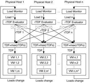
Figure 3.2: TDF controller
In order to synchronize all VHs in the system, virtual time should pass at a same rate in every VH. For this, all VHs in the system should use a common system TDF whose value can adapt to system loads. System loads change the system TDF, and the changed TDF in turn affects system loads, as shown in Fig. 3.2. TheTDF controller dynamically adapts TDF to system loads. Each PH first monitors system loads, which in turn are used to generate their own rTDF. Each PH’s rTDF message is then broadcast to the other PHs in each synchronization interval. The maximum value among all the rTDFs is selected as a new system TDF value, because choosing the greatest rTDF guarantees that VHs which runs on the most heavily loaded physical machine will operate without lagging due to CPU resources. TDF changes in turn causes load changes in the VHs. These load changes are monitored by each PH in the next monitoring interval.
core is utilized and the other cores are idle, the operations of a VH that uses the most heavily-used core can lag behind while the other VHs operate without delay. To make certain that all VHs in a PH operate without delay, the maximum value among all CPU core loads should be taken as the system load.
On one hand, TDF should adapt to current loads as rapidly as possible; on the other hand, the frequency of TDF change should be minimized. In other words, significant changes of system loads should be swiftly reflected in TDF, but their minor oscillations may well be ignored. For emulation accuracy, frequent large changes of the TDF should be avoided, as a large change may not be applied perfectly simultaneously to all VHs, leading to slight timing error in the emulated components.
To resolve these conflicting requirements, the TDF controller uses three parameters: α for the exponential moving average (EMA), Gain, and Insensitivity.
The EMA prevents a change in the current load (Loadcurrent) from changing rT DF too
rapidly. The EMA value of a system load in a monitoring interval, denoted by Load(n), is computed as:
Load(n) = (1−α)·Load(n−1) +α·Loadcurrent. (3.3)
Gain determines how rapidly rTDF will adapt to system loads. If Load(n) is greater than a target load (Loadtarget), rTDF rises, and vice versa. The magnitude of the rising or falling is
directly proportional to the Gain.
Insensitivity minimizes the TDF change unless there is a larger deviation ofLoad(n) from Loadtarget. The required TDF, rT DF(n) is given by:
rT DF(n) =rT DF(n−1)
+Gain·sgn(Load(n)−Loadtarget)
· " " " "
2·Load(n)−Loadtarget
Loadtarget " " " "
Insensitivity
, (3.4)
where sgn(x) is the sign of ×(1 or -1), and |x| is the absolute value of x. The second term in (3.4) has 2 as a scaling factor. A load of 50% is a typical target load. We want the change in the rTDF to be slow when Load(n) is near the Loadtarget but rapid when it is far from
theLoadtarget. We also want rTDF to be approximately linear with respect to Gain when the
Load(n) is around 75%. The scaling factor 2 in (3.4) accomplishes these goals.
will show to work well for a large range of loads.
3.3
System Architecture and Implementation
Synchronization agents exchange control messages (containing rTDFs) to synchronize VHs dis-tributed over different PHs. Each synchronization agent determines the system TDF based on received rTDFs, and if the TDF is changed, each VH immediately applies it. The TDF con-troller of the synchronization agent is tuned so that the rTDF rapidly adapts to system loads, while avoiding the unnecessary minor changes.
3.3.1 Synchronization
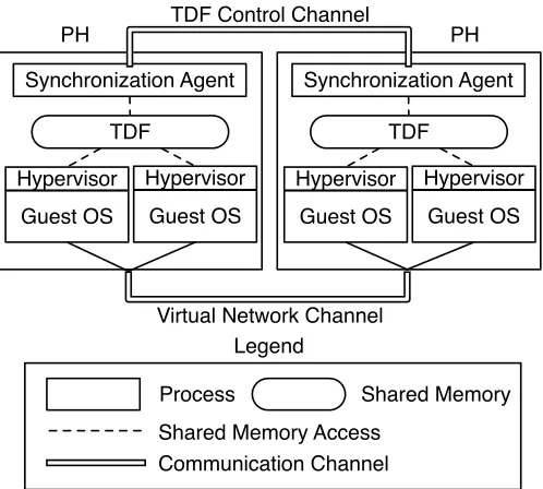
The current TDFs in VHs must be synchronized whether they are colocated in a single PH, or are deployed over multiple PHs. VHs that run on the same PH are locally synchronized through interprocess communications (IPCs) based on shared memory and semaphores, while VHs that are distributed over different PHs are globally synchronized by using UDP packets. For local synchronization, hypervisors on the same PH share a common TDF stored in shared memory, and control their local virtual time based on this TDF value. rTDF values computed by each PH using (3.4) are broadcast via UDP synchronization messages. Synchronization agents are used to compute the current TDF stored in the shared memory and exchange UDP messages.
Fig. 3.3 shows our synchronization method. A synchronization agent periodically generates a required TDF (rTDF) value and broadcasts it to the other PHs. When receiving synchronization messages, each synchronization agent computes a new TDF, which is the maximum of all recently received rTDFs. Thus, all PHs will have a common TDF value upon receiving UDP packets from the other PHs. Virtual time then proceeds at the same rate with a common TDF value in all VHs. To ensure timely dissemination of required TDFs, the synchronization agent periodically generates a new message in a synchronization interval.
VHs running on different PHs can be synchronized with the granularity of the synchroniza-tion interval. So, for example, when testing on our emulasynchroniza-tion system packets’ round-trip time, whose measurement on a real test bed is less than the synchronization interval, the interval can appear to be long. As the synchronization interval decreases, on the other hand, the control messages increase system loads. It is desirable to minimize system loads generated by control messages while maintaining system responsiveness. Hence, a synchronization interval should be carefully chosen, depending on measurement granularity.
Communication Channel Legend
Shared Memory Process
Shared Memory Access Guest OS
Hypervisor
Guest OS Hypervisor
Synchronization Agent PH
TDF
Guest OS Hypervisor
Guest OS Hypervisor
Synchronization Agent PH
TDF TDF Control Channel
Virtual Network Channel
Figure 3.3: The synchronization agent on each PH determines a current TDF and disseminates it to all VHs on that PH.
synchronization delay that network traffic congestion could cause.
Since UDP packets are used for synchronization messages, their loss may cause synchro-nization delay, but synchrosynchro-nization will be rapidly recovered in an interval by the following synchronization message. We deploy our PHs on one LAN and synchronization messages have their own control channels, so there is only a small chance of synchronization delay. Even if a packet loss would occur, since all PHs are in a common broadcast domain, they will usu-ally lose the packet at the same time, so all PHs remained synchronized. TCP would likely have a very large overhead (as it is necessarily unicast vs. the UDP broadcast, and requires acknowledgments), and would introduce additional delays.
3.3.2 Synchronization Agent
Monitor System Loads
Broadcast rTDF
Receive rTDF
Find max rTDF
Notify to Thread 3
Disable virtual time
Suspend VMs
Renew current TDF of shared memory with new max rTDF
Enable virtual time
Resume VMs Wait a
Interval
Thread 2
[notified] Thread 3 Thread 1
[current TDF != max rTDF]
[exit] start
end Compute
rTDF
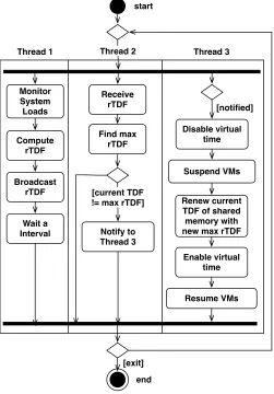
Figure 3.4: Activity diagram of synchronization agent
suspends the operation of all VHs, renews TDF in the shared memory, and resumes VHs. All VMs then operate at a new TDF. In order for the VHs to use virtual time controlled by the synchronization agent, hypervisors must use the TDF of the synchronization agent.
3.3.3 System Tuning
The goal of the dynamic TDF controller of the synchronization agent is to rapidly adapt a TDF value to system loads while avoiding unnecessary changes in TDF. To achieve this goal we must determine appropriate parameter values for α,Gain, and Insensitivity.
measured PH system load used to compute the rTDF, which is broadcast to the other PHs. For the purpose of system tuning, we use a single VH on the PH, so rTDF = TDF.
System performance can be judged by changes in the TDF and CPU loads. Minimizing unneeded TDF variation minimizes changes in TDF across hosts. The degree of TDF oscillation on any PH can be measured by the total summation of the square of the derivatives:
C1 = N−1
!
i=1 #
T DF(i+ 1)−T DF(i) t(i+ 1)−t(i)
$2
, (3.5)
where the summation is taken over a measurement period with N samples. We refer to C1 as
TDF instability.
System overload can be avoided when the current PH CPU loadLoad(i) are close to a target load Loadtarget (50% in our experiments). The oscillation degree of PH loads around a target
can be quantified by:
C2 = %N
i=1(Loadtarget−Load(i))2
N , (3.6)
where the summation is taken over the same measurement period of N. We refer C2 to as
load disturbance attenuation. Anormalized TDF instability C1 is obtained by dividing a TDF
instability by the mean value of all TDF instabilities over a measurement period (i.e., 60 sec. in our experiments), and anormalized load disturbance attenuation C2 is computed by dividing
a load disturbance attenuation by the mean value of all load disturbance attenuations over a measurement period .
The normalizedC1 andC2 are components of cost which are used to minimize TDF changes
as system loads vary. Infrequent and small TDF changes will have less effect on many OS system calls associated with the time passage rate. Some system load fluctuation should be tolerated. Hence, TDF instability is given more weight than load disturbance attenuation and we define total cost as:
C =wIC1+C2, (3.7)
wherewI ≥1 denotes the weight assigned to TDF instability.
The weight wI balances the effects of TDF changes and load response. We choose wI = 10
since the values of Gain and Insensitivity provide responsive systems with modest TDF changes. Experiments showed that wI can vary considerably around 10 without changing near-optimal
system parameters that we will experimentally determine in this section.
0 20 40 60 0 20 40 60 80 100
Square pattern with 10 second period
Real Time (sec)
System Load (%)
(a) Load pattern A
0 20 40 60
0 20 40 60 80 100
Square pattern with 2 second period
Real Time (sec)
System Load (%)
(b) Load pattern B
0 20 40 60
0 20 40 60 80 100
Triangle pattern with 10 second period
Real Time (sec)
System Load (%)
(c) Load pattern C
0 20 40 60
0 20 40 60 80 100
Triangle pattern with 2.5 second period
Real Time (sec)
System Load (%)
(d) Load pattern D
4 8 12 16 20 2 4 6 8 10 0 1 2 3 Insensitivity Gain C1 A
(e)C1A
4 8 12 16 20 2 4 6 8 10 0 1 2 3 Insensitivity Gain C1 B
(f) C1B
4 8 12 16 20 2 4 6 8 10 0 1 2 3 Insensitivity Gain C1 C
(g)C1C
4 8 12 16 20 2 4 6 8 10 0 1 2 3 Insensitivity Gain C1 D
(h)C1D
4 8 12 16 20 2 4 6 8 10 0 1 2 3 Insensitivity Gain C2 A
(i)C2A
4 8 12 16 20 2 4 6 8 10 0 1 2 3 Insensitivity Gain C2 B
(j)C2B
4 8 12 16 20 2 4 6 8 10 0 1 2 3 Insensitivity Gain C2 C
(k)C2C
4 8 12 16 20 2 4 6 8 10 0 1 2 3 Insensitivity Gain C2 D
(l)C2D
4 8 12 16 20 2 4 6 8 10 0 2 4 6 Insensitivity Gain CA
(m)CA= 10C1A+C2A
4 8 12 16 20 2 4 6 8 10 0 2 4 6 Insensitivity Gain C B
(n)CB= 10C1B+C2B
4 8 12 16 20 2 4 6 8 10 0 2 4 6 Insensitivity Gain CC
(o)CC= 10C1C+C2C
4 8 12 16 20 2 4 6 8 10 0 2 4 6 Insensitivity Gain C D
(p)CD= 10C1D+C2D
0 10 20 30 40 50 60
0 1 2 3 4 5 6 7 8 9 10
Real Time (sec)
TDF
Gain = 3, Insensitivity = 4
0 10 20 30 40 50 600
10 20 30 40 50 60 70 80 90 100
System Load (%)
(q) TDF and system load under load pattern A
0 10 20 30 40 50 60
0 1 2 3 4 5 6 7 8 9 10
Real Time (sec)
TDF
Gain = 3, Insensitivity = 4
0 10 20 30 40 50 600
10 20 30 40 50 60 70 80 90 100
System Load (%)
(r) TDF and system load under load pattern B
0 10 20 30 40 50 60
0 1 2 3 4 5 6 7 8 9 10
Real Time (sec)
TDF
Gain = 3, Insensitivity = 4
0 10 20 30 40 50 600
10 20 30 40 50 60 70 80 90 100
System Load (%)
(s) TDF and system load under load pattern C
0 10 20 30 40 50 60
0 1 2 3 4 5 6 7 8 9 10
Real Time (sec)
TDF
Gain = 3, Insensitivity = 4
0 10 20 30 40 50 600
10 20 30 40 50 60 70 80 90 100
System Load (%)
(t) TDF and system load under load pattern D
Figure 3.5: As four patterns of system loads A, B, C, D (a, b, c, d) are offered, the TDF change drives system loads; TDF change is measured by normalized TDF instabilities C1A, C1B, C1C, C1D (e, f, g, h) and load change is measured by normalized load disturbance
attenuations C2A, C2B, C2C, C2D (i, j, k, l); total costs CA, CB, CC, CD (m, n, o, p) are used
rTDF, and the changed rTDF in turn affects the system load in (3.4). Hence, it is extremely complex to find a minimized total cost C, so we rely on measurement rather than introducing a model where the expected value of a linear combination of Gain, Insensitivity, and α is minimized under a randomized experiment plan.
In order to find near-optimal parameter combinations, we analyze how system stability is related to Gain andInsensitivity, as shown in Fig. 3.5. The value ofα for EMA is set to 0.125 so that the oscillations caused by frequent minor variations of loads are removed. The choice
α = 0.125 is analyzed at the end of this section. First of all, square system-load patterns with 10 second period, shown in Fig. 3.5(a), are applied. TDF instability and load disturbance attenuation depend upon Gain and Insensitivity. As shown in Fig. 3.5(e), TDF instability is very high when Insensitivity < 2 regardless of Gain. Otherwise, the effect of Insensitivity is negligible when Insensitivity > ∼3. The normalized load disturbance attenuation gradually increases as Insensitivity grows regardless of Gain, as shown in Fig 3.5(i). For load scenario A, C1A is minimized when Insensitivity > 3, whereas C2A is minimized for smaller values of
Insensitivity. Finally, the total cost (CA = 10C1A+C2A) is depicted in Fig. 3.5(m). Our goal
is to find the combinations of Gain and Sensitivity that approximately minimizeCA.
To accommodate diverse forms of system loads, we repeat the same analysis for additional system load patterns: a square pattern with 2 second period, a triangle pattern with 10 second period, and a triangle pattern with 2.5 second period. These patterns are shown in Fig. 3.5(b), 3.5(c), and 3.5(d). Using the same methodology as for load A, we obtain the total costCB,CC,
CD for load B, C, D as shown in Fig. 3.5(n), 3.5(o), and 3.5(p).
0 1 2 3 4 5 6 7 8 9 10
0 2 4 6 8 10 12 14 16 18 20
Insensitivity
Gain
(a)CA, CB, CC, CD<1.5
0 30 60 90
0 10 20 30 40 50 60 70 80 90 100
Real Time (sec)
System Load (%)
0.1 ms 1 ms 10 ms 100 ms
(b) No VHs
Our goal is to find Gain and Insensitivity that simultaneously minimize CA, CB, CC, and
CD. When a threshold of 1.5 is set for total costs, i.e. CA < 1.5, CB < 1.5, CC < 1.5, and
CD <1.5, the combinations of (1, 4), (3, 4), (4, 6), (2, 9), and (3, 10) are found, as shown in
Fig. 3.6(a).
Even though it is possible to use any combination found in Fig. 3.6(a) in term of system stability, we choose Gain = 3 and Insensitivity = 4, because the combination not only satisfies the cost threshold, but also has rapid responsiveness to load changes (larger Gain and less Insensitivity). Higher Insensitivity decreases TDF changes, but adapts slower to system loads. System loads caused by synchronization messages should be minimized, subject to respon-siveness, so that VHs can maximize the use of their PH’s computing resources. When the synchronization agent runs only in a PH without creating any VHs, the system load increases as a synchronization message interval decreases. This can be seen in Fig. 3.6(b). However, if the synchronization interval ! 10ms, the synchronization messages do not significantly affect system loads. Hence, we choose an update period of 10 ms as a reasonable compromise.
System stability depends onαof EMA as well as Gain and Insensitivity. Smallerαprevents system loads’ large variances from changing TDF too rapidly. As shown in Fig. 3.7(a, b, c), when Insensitivity = 1 and Gain increases from 1 to 3, TDF instability (C1A) increases significantly
withα. As seen in Fig. 3.7(c, d, e, f), asαdecreases and Insensitivity increases from 1 to 4 where Gain is held at 3, TDF instability rapidly decreases. When Insensitivity increases to 3 and α
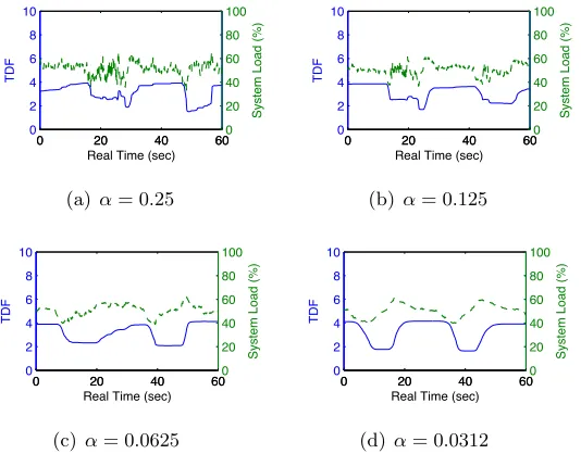
decreases to 0.125 in Fig. 3.7(e), both C1A and C2A become stable. When Gain, Insensitivity ≥3,α= 0.125 stabilizes the system as seen in the pattern of Fig. 3.7(a - f). Values ofα<0.125 (i.e., α= 0.0625,0.0312) also stabilize the system, but decrease responsiveness to system load changes, as shown in Fig. 3.8.
In sum, by using the combination ofGain= 3,Insensitivity= 4,α = 0.125, and a synchro-nization interval of 10 ms, the system can stably operate with rapid TDF response to dynamic system loads, while minimizing TDF changes caused by frequent minor load oscillations.
0.0312 0.0625 0.125 0.25 0.5 1 101 102 103 104 105 α Cost
TDF Instability C1A Load Disturb. Attenuation C
2A
(a) Gain/Insensitivity=1/1
0.0312 0.0625 0.125 0.25 0.5 1 101 102 103 104 105 α Cost
TDF Instability C1A Load Disturb. Attenuation C
2A
(b) Gain/Insensitivity=2/1
0.0312 0.0625 0.125 0.25 0.5 1 101 102 103 104 105 α Cost
TDF Instability C1A Load Disturb. Attenuation C
2A
(c) Gain/Insensitivity=3/1
0.0312 0.0625 0.125 0.25 0.5 1 101 102 103 104 105 α Cost
TDF Instability C
1A
Load Disturb. Attenuation C
2A
(d) Gain/Insensitivity=3/2
0.0312 0.0625 0.125 0.25 0.5 1 102 103 104 105 α Cost
TDF Instability C
1A
Load Disturb. Attenuation C
2A
(e) Gain/Insensitivity=3/3
0.0312 0.0625 0.125 0.25 0.5 1 101 102 103 104 105 α Cost
TDF Instability C
1A
Load Disturb. Attenuation C
2A
(f) Gain/Insensitivity=3/4
Figure 3.7: Effect of exponential moving average coefficient α on our control performance
0 20 40 60
0 2 4 6 8 10
Real Time (sec)
TDF
0 20 40 600
20 40 60 80 100
System Load (%)
(a)α= 0.25
0 20 40 60
0 2 4 6 8 10
Real Time (sec)
TDF
0 20 40 600
20 40 60 80 100
System Load (%)
(b)α= 0.125
0 20 40 60
0 2 4 6 8 10
Real Time (sec)
TDF
0 20 40 600
20 40 60 80 100
System Load (%)
(c)α= 0.0625
0 20 40 60
0 2 4 6 8 10
Real Time (sec)
TDF
0 20 40 600
20 40 60 80 100
System Load (%)
(d)α= 0.0312
3.4
Performance Evaluation
The proposed emulation system is tested by creating distributed VMs and generating streaming traffic, and the heterogeneity and scalability of the system are evaluated.
3.4.1 Experimental Setup
Our emulation system is built on five general purpose servers (Dell PowerEdge R210). Each physical host (PH) has four CPU cores with hyper-threading. Therefore, each host OS recognizes eight CPU cores. In our heterogeneity evaluation, we initially create eight VHs in a PH such that the load of each VH does not greatly affect the other VHs that share a PH. Eight or fewer VHs will have a modest impact on the performance of each other, while more than eight VHs may significantly affect the VHs’ performance. In order to test our system’s scalability, we also load more than eight VHs in a PH during subsequent evaluations.
Each physical machine has two Gigabit Ethernet interfaces connected to different switches. The first interface is used for exchanging synchronization messages and the second interface is used for building a virtual network. VHs in different PHs communicate through the second interface.
Table 3.2: Software packages used in our emulation system.
Linux(PH) ubuntu-10.04-desktop-amd64 Unmodified Linux(VH) ubuntu-10.04-server-amd64 Unmodified FreeBSD FreeBSD-9.0-RELEASE-i386 Unmodified
Windows Windows XP SP3 Unmodified
Junos jinstall-12.1R1.9 Unmodified Hypervisor qemu-kvm-0.13.0 Modified:
307 LOC Sync.
Agent Written from scratch
Created: 2196 LOC
We employ four different OSs, Linux, FreeBSD, Windows XP, and Junos [10, 20], to create the VHs. For virtualization, we use and modify the hypervisor of KVM. KVM’s timer is modified for virtual time, and code for accessing shared memory (where the TDF is stored) is added. Table 3.2 shows details of each software package, including modified lines of code (LOC).
kernel component); Junos can only use TSC and PIT.
We want to be able to have virtual time proceed at a slower rate (as we have seen when the load is heavy) or at a faster rate when the load is light. The first case corresponds to a TDF> 1 and the second case corresponds to a TDF<1. If an experiment generates light system loads, then it can have TDF<1 and virtual time proceeds faster than real time. Thus an experiment with TDF <1 will run on a slower machine but that is advantageous since it will complete in less real time.
3.4.2 Emulation Accuracy
PH2
VH1 PH1
A ping request packet sent every second in virtual time
VH2
(a)
0 1 2 3 4 5 6 7 8 9 10
1 2 3 4 5 10 20 30 40 50 100
Real time [s]
TDF
(b)
0 10 20 30
0.98 0.99 1 1.01 1.02
Virtual time [s]
Inter
−
ping interval [s]
(c)
0 1 2 3 4 5 6 7 8 9 10
1 2 3 4 5 10 20 30 40 50 100
Real time [s]
TDF
(d)
0 10 20 30
0.98 0.99 1 1.01 1.02
Virtual time [s]
Inter
−
ping interval [s]
(e)
For testing emulation accuracy, we measure the inter-ping interval as follows. We set VH1, running on PH1, to send an ICMP echo request packet towards VH2, running on PH2, every second in virtual time, as depicted in Figure 3.9(a). That is, an application running in VH1 sends an ICMP packet and sleeps for one virtual second. When waking up, the application sends the next ICMP packet to VH2.
In order to evaluate our system’s emulation time accuracy under dynamic time dilation, we change the TDF every 100 ms such that the TDF values create a sinusoidal wave between 1 and 100, as seen in Figure 3.9(b). The inter-ping intervals are maintained at approximately one second with less than 2 ms variation in virtual time, as shown in Figure 3.9(c). When the TDF changes every 10 ms and the interval of sinusoidally-changing TDF further decreases as seen in Figure 3.9(d), the inter-ping intervals are still kept around one virtual second with similar variation, as shown in Figure 3.9(e).
3.4.3 Heterogeneity
PH1 PH4
PH2
PH5
PH3
Linux server
Junos router
Windows client
Linux client FreeBSD client OSPF
Physical Host Legend
Figure 3.10: A streaming service topology is created for evaluating heterogeneity.
virtual Juniper routers on PH2 connect the server and the clients running OSPF. While our system supports different OSs on the same PH, we enforce the separation of OSs for simplicity and cleaner system evaluation.
System evaluation is done using a video streaming service similar to the one offered by Netflix [17] and Hulu [8]. The video streaming service loads are approximately constant in the long term (they do vary slightly in the short term), and hence, scale linearly with the number of clients. In our evaluation, we increase the number of streaming clients up to 24 every minute, thus increasing the load on all systems.
To model the video streaming service, the virtual Linux server running on PH1 generates UDP streams at three data rates: 1.5Mbps (corresponding to SD quality), 3Mbps (DVD quality) and 5Mbps (HD quality). The packets are forwarded to the clients by the Juniper virtual routers. Upon receiving a packet each client emulates video decoding by computing a random number a thousand times. In addition to modeling a video streaming service, we also test our emulation system using a real application, the VLC media player [1], in Section 3.4.5.
To evaluate the scaling of TDF with the offered load we add one client every virtual minute (first a Windows client, then a FreeBSD client, then finally a Linux client) until there are 24 clients total (eight of each type). The minimum system TDF is set at 0.01 (i.e, virtual time passes 100 faster than real time). The target CPU load is set at 50%.
0 2 4 6 8 10 10−2
10−1
100
Real Time (min.)
rTDF
Linux server Junos routers Windows clients FreeBSD clients Linux clients
(a) 1.5 Mbps streaming
0 5 10 15 20 25 10−2
10−1
100 101
Real Time (min.)
rTDF
Linux server Junos routers Windows clients FreeBSD clients Linux clients
(b) 3 Mbps streaming
0 10 20 30 40 50 10−2
10−1
100
101
Real Time (min.)
rTDF
Linux server Junos routers Windows clients FreeBSD clients Linux clients
(c) 5 Mbps streaming
Fig. 3.11 shows the required TDF (rTDF) for each of the five PHs for each of the three considered traffic loads. In Fig. 3.11(a) at light loads the PH with the Windows clients experience the largest CPU loads which drives the system TDF from 0.01 to about 0.1. As the number of clients increases, i.e., the traffic forwarded by the routers increases, the load on PH2 (of Junos routers) increases faster than that of PH4 (of Windows clients), further driving the system TDF up to one. When the Linux server generates 3Mbps flows per connection (results shown in Fig. 3.11(b)), the PH generating the largest rTDF changes from the Windows clients (PH4), to the routing PH (PH2) and eventually to the Linux server (PH1). The final TDF at full load, i.e. 24 3Mbps streams, is slightly larger than two. Finally, when the largest streams (5Mbps -shown in Fig. 3.11(c)) are offered, the Linux server quickly becomes the system that drives the overall emulation TDF.
0 1 4 7 10 13 16 19 22 24 0
100 200
Virtual Time (min.)
Received data (MBytes)
FreeBSD 1 FreeBSD 2 FreeBSD 3 FreeBSD 4 FreeBSD 5 FreeBSD 6 FreeBSD 7 FreeBSD 8
(a) 1.5 Mbps streaming
0 1 4 7 10 13 16 19 22 24 0 100 200 300 400 500
Virtual Time (min.)
Received data (MBytes)
FreeBSD 1 FreeBSD 2 FreeBSD 3 FreeBSD 4 FreeBSD 5 FreeBSD 6 FreeBSD 7 FreeBSD 8
(b) 3 Mbps streaming
0 1 4 7 10 13 16 19 22 24 0 100 200 300 400 500 600 700 800 900
Virtual Time (min.)
Received data (MBytes)
FreeBSD 1 FreeBSD 2 FreeBSD 3 FreeBSD 4 FreeBSD 5 FreeBSD 6 FreeBSD 7 FreeBSD 8
(c) 5 Mbps streaming
0 2 4 6 8 10
0 0.2 0.4 0.6 0.8 1 1.2
Real Time (min.)
TDF
(d) 1.5 Mbps streaming
0 5 10 15 20 25
0 0.5 1 1.5 2 2.5
Real Time (min.)
TDF
(e) 3 Mbps streaming
0 10 20 30 40 50
0 0.5 1 1.5 2 2.5 3 3.5 4 4.5
Real Time (min.)
TDF
(f) 5 Mbps streaming
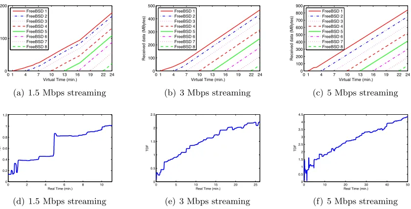
Figure 3.12: The data reception rate in virtual time, i.e. the slope in (a, b, c), maintains near-constant and the value is close to each traffic generation rate (1.5, 3, 5 Mbps), even while TDF is dynamically changing over one order of magnitude.; a stream is added every 3 minutes in virtual time.
The VHs are completely unaware of TDF changes as they change over one order of magni-tude. Fig. 3.12(a, b, c) shows the total amount of data received by the FreeBSD clients while the Linux server generates the packet streams of 1.5 Mbps, 3 Mbps, or 5 Mbps to its clients.
and 5 Mbps respectively. This demonstrates that the VH is truly isolated from changes in TDF. 3.4.4 Scalability PH1 PH2 PH3
...
Linux server Junos router FreeBSD client Physical Host LegendFigure 3.13: A virtual network topology for evaluating scalability.
The virtual network topology shown in Fig. 3.13 is used to evaluate the scalability of our emulation system. The Linux server in PH1 generates a stream of traffic through a Junos router in PH2 to FreeBSD clients in PH3. PH1 creates system loads by generating streaming packets, PH2 by forwarding packets, and PH3 by receiving the packets and emulating video decoding. Each PH generates rTDFs based on the system loads.
In order to evaluate scalability, we increase the VHs (FreeBSD clients) in PH3, so the rTDF from PH3 drives the system TDF. The Linux server in PH1 sends a UDP packet stream to all VHs created in PH3. As the number of VHs increases in PH3, PH3’s system loads increases accordingly.
0 30 60 90 120
1 2 3 4 5 6 7
Real Time (sec)
rTDF
VHs: FreeBSD clients 24 VHs 16 VHs 8 VHs
(a) 3 Mbps streaming
0 30 60 90 120
1 2 3 4 5 6 7
Real Time (sec)
rTDF
VHs: FreeBSD clients 32 VHs 24 VHs 16 VHs
(b) 1.5 Mbps streaming
0 30 60 90 120 1 2 3 4 5 6 7 8
Real Time (sec)
rTDF
2.0 Mbps 1.5 Mbps 1.0 Mbps 0.5 Mbps
(c) 32 VHs in PH3
As more VHs receive a 3 Mbps stream, PH3 creates larger rTDF values as shown in Fig. 3.14(a). When eight VHs are added to the existing eight VHs, the rTDF increases from 1.7 to 3.2, and when eight more VHs are added (total 24 VHs), the rTDF climbs to 6.4. The reason the rTDF increases more from 16 to 24 VHs (3.2) than from 8 to 16 VHs (1.5) is because as more VHs are packed into a PH, context switching and sharing I/O resources require more computing time.
When the server hosts 16, 24 and 32 VHs each generating a 1.5 Mbps stream (total 24,36 and 48Mbps respectively), the rTDF values are shown in Fig. 3.14(b). Compared to the 3-Mbps streaming traffic shown in Figure 3.14(a), the 1.5-Mbps streaming traffic requires a smaller rTDF for the same number of VHs. Even for 32 VHs, the rTDF is approximately 4.8, which is smaller than rTDF≃6.4 for 3-Mbps 24 VHs. As shown in Figure 3.14(c), when we load 32 VHs with 0.5 Mbps of traffic and then increment the traffic load by 0.5 Mbps, the rTDF increases approximately linearly with a slightly larger increase for a larger number of VHs.
3.4.5 Real-world Application: VLC media player
PH2
...
Physical Host LegendVideoLan streaming client (✕ 8)
PH1 VideoLan streaming server
UDP Stream
(a)
0 30 60 90 120
1 2 3 4 5 10 20 30 40 50 100 200
Real Time [s]
TDF
10 Mbps, 1024p, H.264 6 Mbps, 720p, H.264 3 Mbps, 720p, H.264 1 Mbps, 480p, Xvid
(b)
Figure 3.15: (a) A virtual network topology for evaluating the VLC media player that runs on our emulation system (b) Higher video bitrates imply larger TDF.
media player operating as a streaming client, as depicted in Figure 3.15(a).
Table 3.3: Specification of sample video files
File Resolution Codec Video Bitrate
video1 480p Xvid 1 Mbps
video2 720p H.264 3 Mbps
video3 720p H.264 6 Mbps
video4 1024p H.264 10 Mbps
We evaluate our emulation system using four sample video files compressed with different codecs and resolutions. A higher video quality requires a larger bitrate, as seen in Table 3.3. When a single VLC streaming server broadcasts UDP streams to eight VLC streaming clients using the sample video files, PH2, running the VLC streaming clients, is heavily loaded (ap-proaches 100%). Hence, the system load of PH2 drives the system TDF. Since higher quality video streams require more CPU resources for their decompression, the system TDF increases as a video bitrate increases, as shown in Figure 3.15.
3.5
Summary
Chapter 4
Network Link Emulation with
Adaptive Time Dilation
In evaluating the performance of highly complex networked systems, emulation is often used as it maintains much of the realism of testbeds, while offering increased flexibility and scalability. In large emulation systems, multiple and heterogeneous virtual machines can be deployed in relatively few general purpose physical hosts. Time dilation is a technique that allows virtual time to pass at a different (and potentially variable) rate with respect to real time, allowing for increased scalability of the emulated system. In this chapter we present an approach for emulating networking links in a large emulated system employing adaptive time dilation. The link emulation focuses on accurate delay and throughput emulation while allowing varying time dilation factors. To evaluate our system, we measure the delay and throughput of the virtual links under variable system loads.