Octree and Clustering Based Hierarchical Ensemble Visualization.

ABSTRACT

HAO, LIHUA. Octree and Clustering Based Hierarchical Ensemble Visualization. (Under the direction of Christopher G. Healey.)

Interest in ensembles of simulations has increased rapidly in recent years as scientists from various domains use them to assist in their research. An ensemble is a set of results collected from a series of runs of a simulation or an experiment. Each run forms an ensemble member. Ensembles are normally temporal, spatial and contain multiple attribute values at each sample location, making them difficult to analyze or visualize. Techniques have been proposed to provide better insight for a small number of ensemble members, or to present an overview of the entire ensemble but without maintaining fine-grained details. In this paper, we design and implement a system to combine these two directions of ensemble analysis, providing a scalable approach to facilitate analytics of large ensembles and pattern discovery in both the space and the time dimensions.

We begin with a static ensemble analysis and visualization system that focuses on ensemble data at a specific point in time. The static system supports: (1) an octree comparison and clus-tering techniques to provide a hierarchical overview of inter-member shape and data similarity; (2) a glyph-based rendering to create an effective visual representation—a visualization—for a static ensemble member; and (3) a cluster visualization to display similarities and dissimilarities in shape and data value distributions between members.

We then extend the techniques to support analysis and visualization of a temporal ensem-ble, each member encoding data collected from a number of time-steps. The extended system supports two approaches of temporal ensemble analysis.

The first approach provides segment based temporal ensemble analysis, using: (1) member segmentation to combine similar shapes adjacent in a local region in time, thereby improv-ing shape clusterimprov-ing efficiency in large ensembles; (2) segment clusterimprov-ing to combine similar member segments and discover similar shapes in all members across all time-steps; (3) segment cluster abstraction to transform a time-series member into a sequence of clusters of member segments; (4) closed contiguous item sequential pattern mining (CISP) over the member cluster participation sequences to identify frequent contiguous changes in shape over time; (5) dynamic time warping (DTW) and time-series member clustering to generate a hierarchical overview of relationships between time-series members, respecting changes in shape over time that include possible shifting and distorting in the time dimension; and (6) animation-based extensions to visualize changes in shape over time.

This approach is an extension of the static ensemble analysis, using: (1) hierarchical cluster-ing to combine similar shapes at every time-step; (2) time-step shape cluster abstraction to transform a time-series member into a sequence of time-step shape clusters; (3) CISP in the time-step shape cluster participation sequences to discover common shape changes in the ensem-ble; (4) Manhattan distance member comparison and time-series member clustering to provide a hierarchical overview of inter-member relationships; and (5) the same animation technique to visualize a time-series member cluster or a pattern.

© Copyright 2015 by Lihua Hao

Octree and Clustering Based Hierarchical Ensemble Visualization

by Lihua Hao

A dissertation submitted to the Graduate Faculty of North Carolina State University

in partial fulfillment of the requirements for the Degree of

Doctor of Philosophy

Computer Science

Raleigh, North Carolina

2015

APPROVED BY:

Robert St. Amant Russell M. Taylor II

Steffen A. Bass Christopher G. Healey

BIOGRAPHY

Lihua Hao was born and grew up in Qiqihar, the second largest city in Heilongjiang province, People’s Republic of China. She received her Bachelor of Science degree in Computer Science from Peking University, Beijing, China in 2010. In the same year, she joined the doctoral program in Computer Science at North Carolina State University.

ACKNOWLEDGEMENTS

I would like to express my deep appreciation and gratitude to Dr. Christopher G. Healey, my advisor, for the initiation of my research and for his guidance, encouragement and patience during my graduate studies at North Carolina State University. I appreciate his contributions in time and efforts. I could not have imagined having a better advisor and mentor for my Ph.D. study. I would like to thank Dr. Steffen A. Bass for providing the Relativistic Heavy Ion Collision (RHIC) ensemble to validate my research, helping me learn about the RHIC data and inspiring me on improving my work. I would like to thank my other committee members, Dr. Russell M. Taylor II, Dr. Randy Avent, Dr. Subhashish Bhattacharya and Dr. Roberts St. Amant, for giving me insightful comments and suggestions on my research.

My sincere thanks also goes to Dr. Andy Wilson, my supervisor during my summer intern-ship at Sandia National Laboratories (SNL) in 2012. He provided me the opportunity working on the metal ball collision ensemble data at SNL and offered me insightful comments and sug-gestions on my work. I would like to thank Dr. Warren Leon Davis at SNL for helping me improve the clustering algorithms in my research. I thank all my friends in the Knowledge Discovery Lab for the stimulating discussions and for all the fun we had in the last four years.

TABLE OF CONTENTS

LIST OF FIGURES . . . vi

Chapter 1 Introduction . . . 1

Chapter 2 Background. . . 5

2.1 Volume Rendering . . . 5

2.2 Multidimensional and Multivariate Visualization . . . 7

2.3 Comparative Visualization . . . 10

2.4 Dynamic Time Warping . . . 13

2.5 Sequential Pattern Mining . . . 15

2.6 Ensemble Visualization . . . 16

Chapter 3 Relativistic Heavy Ion Collision Ensemble . . . 23

Chapter 4 Static Ensemble Analysis . . . 25

4.1 Octree Representation for 3D Shape . . . 26

4.2 Shape Dissimilarity Measurement . . . 27

4.3 Cluster Tree Visualization . . . 30

4.3.1 MST Based Clustering . . . 30

4.3.2 Agglomerative Clustering . . . 32

4.4 Visualization . . . 34

4.4.1 Single Member Visualization . . . 34

4.4.2 Cluster Visualization . . . 35

Chapter 5 Temporal Ensemble Analysis. . . 39

5.1 Octree Construction . . . 44

5.2 Cluster Shape Dissimilarity Measure . . . 44

5.2.1 Group Average Linkage . . . 45

5.2.2 Octree Shape Integration Based Dissimilarity Measure . . . 45

5.3 Member Segmentation . . . 46

5.3.1 Contribution Ratio Based Member Segmentation . . . 46

5.3.2 Shape Integration Based Member Segmentation . . . 48

5.4 Time-Series Member Clustering . . . 50

5.5 Segment Based Shape Clustering . . . 52

5.6 Segment Cluster Abstraction . . . 54

5.7 Member Cluster Participation Pattern Mining . . . 56

5.8 Temporal Visualization . . . 62

Chapter 6 Time-Step Ensemble Analysis . . . 65

6.1 Time-Step Member Clustering . . . 65

6.2 Time-Series Member Clustering . . . 67

6.3 Time-Step Shape Based Pattern Mining . . . 68

Chapter 7 RHIC Application . . . 70

7.1 Ensemble Analysis System . . . 72

7.2 Segment Based Ensemble Analysis . . . 72

7.3 Time-Step Based Ensemble Analysis . . . 76

Chapter 8 Conclusion . . . 83

8.1 Strengths . . . 83

8.2 Limitations . . . 84

8.3 Future Work . . . 85

LIST OF FIGURES

Figure 2.1 An object-order and obscurance-based volume rendering framework applied to a CT-human body data set [36], to display inner structures of the data in addtion to the two dimensional surface . . . 6 Figure 2.2 Ray casting for image-based volume rendering . . . 6 Figure 2.3 Surface glyph visualization of hurricane Isabel, temperature, precipitation

and air pressure are mapped to the color, thickness and roundness parameters of the glyphs [35] . . . 8 Figure 2.4 Parallel coordinates for a seven dimensional “cars” dataset with 392 data

points, color indicates clusters of data point and histogram bars highlight point distributions along the axes [26] . . . 9 Figure 2.5 Variable binned scatter plots showing correlations between credit card fraud

amounts [14] . . . 9 Figure 2.6 Two comparative visualization approaches: (a) image level comparison

com-pares visual impressions of raw data; (b) data level comparison displays the results of a comparison between the original data sets or features of original data sets . . . 11 Figure 2.7 Comparisons between intersecting surfaces [44]. The two surfaces on the left

are used to produce the visualization on the right. Internal surface regions are rendered as neutral gray material with a regular-grid texture colored by the surface that is exterior at the texture’s position. Exterior surface regions appear as glyphs, i.e., simple elongated pluses with their long axes indicating estimates of the first principal curvature directions at the glyph centers . . . 12 Figure 2.8 (a) Euclidean distance aligns elements in two time series “one to one”,

pro-ducing a poor dissimilarity score; (b) Dynamic Time Warping produces a more intuitive dissimilarity measure with non-linear alignment, allowing sim-ilar shapes to match even if they are out of phase in the time dimension . . . 14 Figure 2.9 Global constraints such as (a) Sakoe-Chiba band and (b) Itakura

parallelo-gram are applied to speed up the DTW algorithm by restricting the matrix of elements that a warp path is allowed to visit . . . 15 Figure 2.10 The Ensemble-Vis framework provides a platform for data visualization and

analysis through a combination of statistical visualization techniques and high level user interaction [34] . . . 17 Figure 2.11 Quartile trend charts in Ensemble-Vis show the quartile range of the ensemble

within a user-selected region. The minimum and maximum are shown in blue, the gray band shows the 25th and 75th percentiles, and the median is indicated by the thick black line . . . 18 Figure 2.12 Plume trend charts in Ensemble-Vis show the average of each ensemble model

Figure 2.13 An illustrative ensemble visualization in Noodles [40]: (a) graduated uncer-tainty glyphs spread over the entire grid calculated for perturbation pressure; (b) graduated glyphs along the perturbation pressure contour of the ensem-ble mean; (c) uncertainty ribbon for perturbation pressure with a colormap of the ensemble standard-deviation . . . 19 Figure 2.14 Ensemble surface slicing (right image) applied to four static ensemble

mem-bers (left four images) for comparative visualization [3] . . . 20 Figure 2.15 3D visualization of three simulated ensemble members—apple, banana and

pear [31]: (a) pairwise sequential animation visualizes multiple members by varying their opacity visibilities; (b)screen door tinting chooses the apple as the reference member and shows differences between members with a yellow tint for the banana, an orange tint for the pear and gray for regions in the apple that do not overlap either member . . . 20 Figure 2.16 Overview of the system designed by Piringer et. al. [32]: (a) the

member-oriented overview employing feature-based placement (b) for 524 2D func-tions; (c) the mid-level focus of 31 selected members; (d) the domain-oriented overview showing the point-wise range of the selected subset; (e) the 3D sur-face plot of a single member . . . 21

Figure 3.1 The calculated transition from ordinary nuclei to free quarks and gluons. The protons and neutrons within the nuclei are disintegrated at extremely high temperature or density, liberating quarks and gluons. RHIC collisions are expected to reach this regime, albeit briefly [27] . . . 24

Figure 4.1 Building an octree to represent a 3D mesh model . . . 26 Figure 4.2 Octree-based hierarchical spatial subdivision . . . 26 Figure 4.3 Two clustering techniques applied in our system: (a) a top-down MST based

clustering; (b) a bottom-up agglomerative clustering . . . 30 Figure 4.4 MST cluster tree showing hierarchical clustering results of 20 members, red

nodes highlighting clustering results withk= 7 or σ= 0.21 . . . 31 Figure 4.5 Agglomerative cluster tree visualizes hierarchical clustering results of 20

members, red nodes highlighting the clustering result defined by k = 5 or

σ= 0.23 . . . 32 Figure 4.6 Agglomerative clustering results whenk= 5 . . . 33 Figure 4.7 Single member visualization at different levels of detail: (a) all leaf octants;

(b) a more abstract cutoff level . . . 36 Figure 4.8 (a) The cluster visualization (cluster 35 in in Figure 4.5) of four members:

(b) member 5, (c) member 15, (d) member 18 and (e) member 20 . . . 38

Figure 5.1 Procedure of time-series member clustering that products a hierarchical overview of inter-member relationships in a temporal ensemble. . . 40 Figure 5.1 Procedure of time-series member clustering that products a hierarchical overview

of inter-member relationships in a temporal ensemble. . . 41 Figure 5.2 Procedure to discover important patterns that occur across multiple members

Figure 5.2 Procedure to discover important patterns that occur across multiple members in a temporal ensemble . . . 43 Figure 5.3 A color image segmentation example: (a) original color image of a picture of

poppy (b) result after color segmentation . . . 47 Figure 5.4 A time-series member with 60 time-steps are combined into 11 segments

by shape integration based member segmentation with maximum median distance of 0.4 . . . 49 Figure 5.5 DTW member agglomerative cluster tree according to the DTW time-series

member dissimilarities (a) segment median distance = 0.4 (b) segment me-dian distance = 0.35 . . . 51 Figure 5.6 Segment cluster tree visualization of the 62 segments for a six member RHIC

ensemble, red cluster nodes highlighting the clustering result determined by

k= 16 orσ= 0.3 . . . 53 Figure 5.7 Threshold of all clustering results encoded in Figure 5.6 . . . 53 Figure 5.8 IDs of the 16 clusters highlighted in Figure 5.6 and the segments each cluster

contains . . . 54 Figure 5.9 An example of segment cluster abstraction. Time series member M1 is first

transformed into a sequence of member segmentsM S1 = (ms1, ms2, ..., ms10), and then transformed into a member cluster participation sequenceCS1, by mapping each segment to its corresponding segment cluster in Figure 5.8 . . 55 Figure 5.10 Segment cluster abstraction transforms the time-series members to sequences

of member segments, then to member cluster participation sequences based on Figure 5.8 . . . 55 Figure 5.11 The MSFSIS collections of cs108 . . . 57 Figure 5.12 (a) Down Trie compressed to (b) Down Tree representing the MSFIS

collec-tion of 108 in Figure 5.11 . . . 58 Figure 5.13 The UpDown Tree of 108 (root node A) representing the MSFSIS collection

of 107 in Figure 5.11 . . . 58 Figure 5.14 Closed CISP mining result of the member cluster participation sequence set

in Figure 5.10, minimum support = 4 . . . 63 Figure 5.15 The two closed CISPs that occur in all members . . . 63 Figure 5.16 Visualization of a time-series member fades in and out each member item

based on their orders in time-steps, the slider value indicating current visible time-step . . . 64

Figure 6.1 Maximum (blue line) and average (red line) thresholds at all time-steps. . . . 66 Figure 6.2 Number of clusters at all time-steps, σ= 0.2. . . 66 Figure 6.3 Agglomerative Manhattan distance member cluster tree . . . 67 Figure 6.4 Patterns discovered according to time-step shape cluster participation

se-quences, minimum support = 4 . . . 68 Figure 6.5 Red areas highlight time regions covered by patterns that occur (a) in all

Figure 7.1 Our stand-alone ensemble visualization system, with a single 3D OpenGL widget on the left and a user interface on the right to control visualization and ensemble analysis . . . 70 Figure 7.2 The user interface consists of (a) a display widget to control visualization (b)

an analysis widget to control temporal ensemble analysis and (c) an octree widget to control octree comparison and visualization . . . 71 Figure 7.3 The ensemble overview widget represents the 41-member, 60 time-step

en-semble with 41_×60 grids. Member items belonging to selected segments, clusters, patterns or members will be highlighted in red upon scientists’ re-quirements . . . 71 Figure 7.4 (a) Member segmentation results, each red rectangle representing a member

segment. Segment connections in the dashed rectangle discover the time-steps when the cylinder shape starts to break into two dumb bell sides, e.g., (a)

t48 to (b)t49 inM3 and (c) t49to (d) t50 inM5 . . . 74 Figure 7.5 (a) Visualization of the agglomerative segment cluster tree, displaying only

clustering results with k_≤100; (b) thresholds of all segment clustering results 75 Figure 7.6 All 5 segment patterns with support_≤40 (selected patterns in the right list) 76 Figure 7.7 Member cluster participation pattern 4 consists of three clusters of segments:

cs1058, cs1050, cs1044 . . . 77 Figure 7.8 (a) Segment based time-series member cluster tree. (b) Thresholds of all

clustering results encoded in the cluster tree . . . 78 Figure 7.9 (a) Cluster tree visualization at time-step 50, two red nodes highlighting

clustering result with k= 2 clusters: (b) cluster 70 and (c) cluster 80. . . 79 Figure 7.10 (a) Time-step comparison based member cluster tree. (b) Thresholds of all

Chapter 1

Introduction

Visualization is “the use of computer-supported, interactive, visual representations of data to amplify cognition” [8]. It converts data into a visual form like an image or an animation to support rapid and effective comprehension of large amounts of information. This enables viewers to discover patterns that might otherwise be buried in traditional numerical forms. As computing power has increased, the size and complexity of the data being collected has accelerated, producing a corresponding increase in the time and effort needed for data analysis. It is often too difficult for humans to mentally aggregate their data to identify important patterns based entirely on numerical forms, even with automatically derived aggregates. This problem prompted researchers to consider analyzing data through the use of visualization. Since its inception in an NSF report [25] in 1987, visualization has gradually become a highly interdisciplinary field with positive impacts in areas like medicine [23], scientific research [31, 34] and business decision-making [15]. A broad classification places visualization techniques into two categories [8]: scientific visualization and information visualization. The former is applied to scientific data, which are often physically based numerical data; while the latter is applied to abstract data, which are often not physical based.

of terabytes. It is extremely difficult to create a generalized visualization of this type of dataset, not only due to limitations of memory and screen space, but also because our visual system cannot interpret such an overwhelming amount of information. Ensembles normally contain numerous data attributes (e.g., variable, space, member and so on), necessitating some type of multivariate visualization, itself a challenging task. Unlike traditional scientific data analysis which usually works with a single simulation, ensemble analysis focuses on exploring inter-member relationships, so comparison is crucial. Furthermore, many ensembles are temporal (i.e., each member contains shapes, values and events that vary over time), requiring some type of time-series or sequential data mining to support analysis of their dynamic characteristics.

A number of techniques have been developed for ensemble analysis and visualization. Some of them [10][34] rely on statistical methods to support ensemble summarization. Displaying the concise results of complex analysis or sampling is comparatively simple, but omits potentially important details in the original data. Other approaches [3][31] are inspired by traditional sci-entific visualization techniques that aim to provide better insights for a single simulation. These approaches are extended to support comparison between members. This provides a better view of the individual members, but often limits comparison to only a small, static member set. Described this way, the two main approaches to ensemble visualization either provide: (1) an ensemble overview that scales but does not maintain fine-grained details, or (2) a multivariate visualization that maintains detailed information but only handles a few members at a time. More recently, advanced systems [24][32] have been designed to support interactive visual anal-ysis of an ensemble at different levels of detail. These systems rely on scientists to define a subset of members for detailed visualization by brushing in a high level ensemble view. Little work has been done to automatically capture inter-member relationships or to explore patterns in the time dimension.

(i.e., averages and variances) with a visual result that highlights shape and data differences through the use of size and animation. In this way, we extend traditional multivariate visual-ization to support general shape visualvisual-ization and region-by-region comparative visualvisual-ization across multiple ensemble members. This provides a detailed view of shape, data distribution and important data value differences across the members in a cluster.

Next, we extend the system to support analysis and visualization of temporal ensembles. The extended system supports two approaches of temporal ensemble analysis—a segment based approach and a time-step based approach.

The segment based approach combines similar shapes from all members across all time-steps. We initially transform each time-series member to a sequence of member segments by combining member items with similar shapes that lie in a local region in the time dimension. We apply dynamic time warping (DTW) [41] to compare time-series members based on their changes in shape over time. DTW results are used to build a cluster tree that reveals hierarchical inter-member relationships in the temporal ensemble. To explore common shapes that occur at discontinued time-steps and across members, we cluster the member segments over the entire ensemble. We then transform the ensemble into a set of member cluster participation sequences according to a user-selected number of clusters of member segments. We adapt the UpDown trees contiguous item sequential pattern (CISP) mining[9] to discover patterns in the member cluster participation sequences. The resulting patterns identify contiguous shape changes that occur frequently in the ensemble. We extend our multivariate visualization to display patterns and time-series member clusters, using animations to fade in and out a sequence of visualizations ordered in time.

The second approach, time-step ensemble analysis, is motivated by our physics collabora-tors’ particular research interest in comparing members at every time-step. This approach first clusters members at each time-step independently as in static ensemble analysis. This converts the ensemble into a set of time-step shape cluster participation sequences suitable for a closed CISP mining. We apply Manhattan distance to compare time-series members by averaging dissimilarities at all time-steps.

The pattern mining, hierarchical clustering and member visualization techniques are em-ployed to discover important features in the time dimension and inter-member relationships. Our segment based approach is capable of time-length reduction and optimal match finding. The time-step based approach performs member relationship analysis at every time-step to capture more detailed pattern sequences. The two approaches enables scientists to visualize and analyze a temporal ensemble from different perspectives at different levels of detail.

The main contributions of our work include:

ensemble visualizations, exemplified with a heavy ion collision ensemble generated by nuclear physicists at Duke University.

2. Octree representations to encode spatial shape, reduce data size and mathematically com-pare static ensemble members.

3. Dynamic time warping or Manhattan distance to mathematically compare time-series members with or without shifting and distorting in the time dimension.

4. A cluster tree visualization that provides an overview of hierarchical inter-member rela-tionships in a static or temporal ensemble prior to the need for detailed visual comparisons.

5. A member segmentation to efficiently combine similar shapes from a local time region, to capture important shape transitions and simplify shape clustering and member visualiza-tion in a temporal ensemble.

6. An adaption of UpDown tree contiguous item sequential pattern mining to identify con-tiguous changes in shape that occur frequently in a temporal ensemble.

7. A cluster visualization to compare shape and data values of multiple static members, enabling scientists to investigate different clustering results.

Chapter 2

Background

This chapter provides an overview of previous research related to analysis and visualization of ensemble data, and describes their applications in existing ensemble visualization approaches. We explicitly focus on the techniques that inspired our ensemble visualization system, each of which addresses certain challenges of three dimensional ensemble visualization or temporal data analysis. Volume rendering provides visual insight for 3D volumetric data sets; multi-dimensional visualizationprojects high-dimensional data into 2D or 3D space while maintaining key features of the original data;comparative visualization highlights differences and similarities between large datasets through the use of visualization;dynamic time warping uses time-series data mining to identify optimal alignments of temporal data value changes; sequential pattern mining discovers patterns that occur frequently in a set of sequences ordered in time. A number of frameworks and techniques have been designed and applied to facilitate interpretation and analysis of 2D or 3D ensembles in different scientific domains.

2.1

Volume Rendering

Figure 2.1: An object-order and obscurance-based volume rendering framework applied to a CT-human body data set [36], to display inner structures of the data in addtion to the two dimensional surface

ensemble.

Volume rendering techniques are classified into three categories [19]: image-order, object-order and domain-based object-order. Image-order volume rendering, such as x-ray rendering, casts rays through each pixel into the volume (Figure 2.2), and calculates a final pixel value by aggregating contributions of voxels along the ray with a transfer function.Object-order volume rendering, such as splatting [11], differs from image-order rendering by projecting each voxel individually onto the screen to create final image. An object-based approach is more efficient if large empty spaces exist, because it only stores voxels within the object that contain data.

Domain-based volume rendering transforms data into another domain (e.g., wavelet domain [45]) before ray casting, to take advantage of useful features in the intermediate domain.

2.2

Multidimensional and Multivariate Visualization

The terms multidimensional and multivariate are often used interchangeable in the visualization literature [47]. In this paper, dimension refers to physical dimensions of the data, i.e., space and time, while variate refers to the non-physical data attributes. Multidimensional visualiza-tion projects data with high dimensionality into a 2D or 3D display, while maintaining key features of the original data. Multivariate visualization focuses on displaying the distributions and relationships of the non-physical attributes.

Multidimensional visualization techniques consider the spatial and temporal embedding of data. A large number of techniques have been proposed to project 3D spatial data to 2D space. For example, volume rendering (Section 2.1) creates 2D images for 3D volumetric data, capturing both the external surfaces and internal structures. A technique named Grand Tour [49], projects high dimensional data onto a sequence of 2D planes, and traverses from one projection to the next to gain a multi-sided view of the original data. Statistical projection techniques such as multidimensional scaling (MDS) [7] or principal component analysis (PCA) [5] map high dimensional data to a 2D subspace while maintaining distance or variance between data points. If a time dimension exists, animation, such as flickering, may be applied to display temporal coherence in the data.

Figure 2.4: Parallel coordinates for a seven dimensional “cars” dataset with 392 data points, color indicates clusters of data point and histogram bars highlight point distributions along the axes [26]

resent multiple attributes as parallel vertical bars. The domain of each attribute is mapped to positions along its bar (e.g., bottom-to-top for an ordinal attribute). Each data element forms a polyline that connects the position of each of its attribute values on adjacent coordinate axes. A dataset forms a collection of polylines whose shape and density highlight patterns and distributions of attribute values in the dataset. Parallel coordinates focus mainly on analysis of relationships between adjacent coordinates. Figure 2.4 illustrates the use of parallel coordi-nates to display a 392-point “car” dataset with seven attributes. Each vertical axis represents an attribute (e.g., weight, year, origin) in the dataset, and attribute values in each data point are connected by a polyline. Polylines are colored to highlight clusters of cars with common properties. Another example, variable binned scatter plots [14] (Figure 2.5) combines a group of related scatter plots, a well-known data analysis chart for displaying relationships between pairs of attributes, to show relationships across multiple attributes.

There is no obvious division between multidimensional and multivariate visualization. Even though it is less common, each dimension can be treated as an attribute and used in a multi-variate visualization to display relationships between dimensions. An ensemble data set is often both multidimensional and multivariate, requiring the combination of both types of techniques.

2.3

Comparative Visualization

Comparison is a key procedure to verify and analyze scientific simulations [2]. Comparative vi-sualization highlights similarities and differences between large data sets. A broad classification places comparative visualization techniques into two categories [29]: image level comparison and data level comparison.

data set 1

data set 2

visualization pipeline

visualization pipeline

image fusion Image

(a)

data set 1

data set 2

data conversion

data conversion

visualization pipeline Image

compare

(b)

Data level comparison [21] directly compares the original data sets, then creates a visual-ization of the results (Figure 2.6b). Figure 2.7 illustrates a data level comparison between two intersecting surfaces. Data level comparison supports more in-depth comparative analysis. It allows scientific operations to be applied to the raw data or their extracted features to highlight differences or similarities. A major limitation of data level comparison is a lack of generality, since the metrics required for raw data comparison vary greatly between different applications. In ensemble analysis, scientists are often interested in similarities and differences, for exam-ple, between different members or between time-steps within a member. Comparative visualiza-tion has been adopted in various ensemble visualizavisualiza-tion frameworks. For example, [34] supports side-by-side comparison across multiple linked views, and [31] applies flicker to compare mul-tiple 3D spatial ensemble members. Our ensemble visualization technique supports data-level comparison of shapes and attribute distributions between members.

2.4

Dynamic Time Warping

Time series data is collected in many domains such as molecular biology, meteorology, astro-physics and manufacturing. A time series is a set of values or events that vary over time. Choosing an appropriate dissimilarity measure that respects the continuous nature of a time series is a fundamental requirement in time series mining. A simple dissimilarity measure can provide unintuitive results if two time series have similar overall shapes but the shapes do not align exactly in the time dimension (Figure 2.8a). Dynamic Time Warping (DTW) [41] overcomes this limitation by finding an optimal non-linear alignment that ignores shifting and distortion in the time dimension (Figure 2.8b). It has been widely applied in various time series mining tasks including clustering, classification, pattern recognition and motif discovery.

DTW finds an optimal match between two time series by minimizing their dissimilarities. Given time series Si = (ti1, ti2, ..., tin) and Sj = (tj1, tj2, ..., tjm), DTW constructs an n×m

matrix where the (p, q) element of the matrix is dissimilarity d(p, q) between tip and tjq. The

optimal alignment is determined by the shortest warping path in the matrix that minimizes dissimilarity betweenSiandSj. A warping path,W =w1w2...wK,max(m, n)≤K≤m+n−1,

is a set of contiguous matrix elements that defines a mapping betweenSi andSj, satisfying the

following three constraints:

(1) boundary: the warping path must start at w1 = (1,1) and end at wK = (n, m);

(2) continuity: the warping path must advance one step at a time, i.e., p _≤ p0 _≤ p+ 1 and

q ≤q0 ≤q+ 1 for anywk = (p, q) andwk+1 = (p 0

, q0);

(3) monotonicity: the warping path must not roll back, i.e., p0 ₋p_≥0 and q0₋q _≥0 for any

wk= (p, q) and wk+1 = (p 0

, q0).

Dissimilarity between Si and Sj along warping path W is defined asdW =PK_k=1d(wk) where

d(wk) =d(p, q) ifwk = (p, q). Calculating the DTW dissimilarity of Si and Sj is equivalent to

finding the shortest warping path, mathematically,

DT W(Si, Sj) = min W

( _K X

k=1

d(wk)

)

. (2.1)

DTW uses dynamic programming to calculate DT W(Si, Sj). Let D(p, q) be the distance

along the shortest warping path of prefix time series S_i0 = (ti1, ti2, ..., tip), 1≤p≤n, of Si and

S_j0 = (tj1, tj2, ..., tjq), 1≤q ≤m, ofSj, then D(p, q) is equivalent to the dissimilarity between

tip andtjq plus the minimum dissimilarity of the optimal warping paths of the time series that

are one step ahead, meaning

(a) (b)

Figure 2.8: (a) Euclidean distance aligns elements in two time series “one to one”, producing a poor dissimilarity score; (b) Dynamic Time Warping produces a more intuitive dissimilarity measure with non-linear alignment, allowing similar shapes to match even if they are out of phase in the time dimension

The DTW dissimilarity of Si and Sj is

DT W(Si, Sj) =D(n, m). (2.3)

The conventional DTW algorithm has O(mn) time and space complexity. Derivative algo-rithms have been proposed to improve its performance as well as to reduce the space overhead. Global constrains such as the Sakoe-Chiba band [37] and the Itakura parallelogram [16] (Fig-ure 2.9) are proposed to slightly improve the calculation and to prevent pathological warpings by restricting the subset of matrix elements that the warping path is allowed to visit. The per-formance of a global constraint-based DTW algorithm relies on the size of a restricted region in the matrix. Accuracy of the dissimilarity measure may not be guaranteed if the optimal warping path traverses cells outside the constraint region. Other approaches use data abstrac-tion to perform DTW on an abstract representaabstrac-tion of the original time series. The abstracabstrac-tion level has to be chosen carefully. An abstraction that is too fine may provide little performance improvement, while an abstraction that is too coarse may produce an inaccurate optimal warp-ing path. Multi-scale approaches such as FastDTW [38] recursively project an optimal warpwarp-ing path found at a lower resolution to the next higher level and then refine the projected path through local adjustments. FastDTW has a linear space and time complexity and provides a reasonable approximation of the optimal warping path. In some particular tasks such as time-series classification or pattern finding, indexing techniques are applied to reduce the number of times DTW is run, rather than speeding up the actual algorithm.

(a) (b)

Figure 2.9: Global constraints such as (a)Sakoe-Chiba band and (b)Itakura parallelogram are applied to speed up the DTW algorithm by restricting the matrix of elements that a warp path is allowed to visit

time. Dynamic Time Warping enables us to statistically measure dissimilarity of the continuous changes in shape or attribute values between time-series members, so that we can better explore inter-member relationships of the ensemble while respecting data variation over time.

2.5

Sequential Pattern Mining

Sequential pattern (SP) mining discovers the complete set of frequent subsequences as patterns in a set of sequences S. Each sequence consists of an ordered list of itemsets and each itemset consists of a non-empty set of items. A sequence s0 =< s0₁, s0₂, ..., s0_m > is a subsequence of another sequence s =< s1, s2, ..., sn >, i.e., s a super-sequence of s

0

, if there exist integers 1≤i1< i2 < ... < im ≤nso that s

0

1 ⊆si1,s

0

2⊆si2, ...,s

0

m⊆sim. A subsequence is considered frequent if its occurrence in _S is no less than a user-specified threshold minSupport.

be infrequent.Pattern-growth based approaches, such as FreeSpan [13] and PrefixSpan [30], use a depth-first traversal procedure that recursively projects a sequential database into a set of smaller databases based on frequent patterns mined to date. Patterns in the projected databases are expanded based on the apriori principle. Pattern-growth based approaches avoid the ex-pensive candidate generation and evaluation step in apriori-based approaches by focusing on a small portion of the original database in each iteration, but it may still be costly to recursively generate a large number of projected databases.

At an application level, the problem of SP mining might be too general, meaning a user may only be interested in a subset of patterns with specific features.Contiguous item sequential pattern (CISP) mining requires each sequence to be an item sequence and each pattern to be a contiguous subsequence. A sequence is an item sequence if it consists of an ordered list of single items. A subsequence is contiguous if its items appear adjacent to one another. Simply adapting general SP mining techniques to CISP mining could be inefficient both in time and memory due to the size of the search space. Because of this, algorithms have been proposed to utilize specific constraints of CISP to reduce the search space and improve pattern mining performance. For example, Zhang et. al. [18] proposed a CISP-Growth algorithm for analysis of application level IO patterns. This algorithm preforms only one scan of the original sequence to construct a linear array of slices, then grows patterns among the slices. Chen [9] proposed a data structure called an UpDown tree—a combination of two tree structures sharing the same root—to efficiently capture prefixes and suffixes of an itemsi represented by the root node. The

problem of CISP mining is decomposed to efficient mining of a collection of disjoint subsets of CISPs based on a series of UpDown trees. Experimental results in [9] indicate that Chen’s algorithm outperforms widely-used general SP mining techniques for web log pattern mining.

In a time-series ensemble, each member is a sequence of member items ordered in time and collected from one run of a simulation or an experiment. By considering similar member items as identical sequence items, we can adapt CISP mining to discover similar contiguous changes in shape that frequently occur in the ensemble.

2.6

Ensemble Visualization

Figure 2.10: The Ensemble-Vis framework provides a platform for data visualization and anal-ysis through a combination of statistical visualization techniques and high level user interaction [34]

comparative visualization.

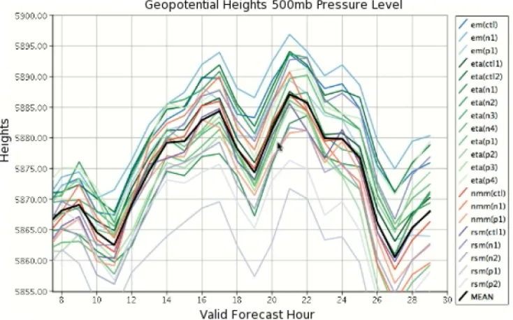
Figure 2.11: Quartile trend charts in Ensemble-Vis show the quartile range of the ensemble within a user-selected region. The minimum and maximum are shown in blue, the gray band shows the 25th and 75th percentiles, and the median is indicated by the thick black line

(a) (b) (c)

Figure 2.13: An illustrative ensemble visualization in Noodles [40]: (a) graduated uncertainty glyphs spread over the entire grid calculated for perturbation pressure; (b) graduated glyphs along the perturbation pressure contour of the ensemble mean; (c) uncertainty ribbon for per-turbation pressure with a colormap of the ensemble standard-deviation

Noodles [40] is another visualization tool built for analysis of meteorological ensembles. Similar to Ensemble-Vis, it supports interactivity, multiple linked views, spaghetti plots, and use of mean and standard deviation. Furthermore, it provides more complex statistical aggre-gation and uncertainty measurements such as inter-quartile ranges, 95% confidence intervals and bootstrapping means. Noodles employs circular glyphs and ribbons for ensemble visualiza-tion. Glyphs are spread over grids (Figure 2.13a) or along a contour of means (Figure 2.13b). The glyph’s appearance (i.e., size, density and saturation) visualizes deviations from the mean and differences across members. An uncertainty ribbon walks along a contour with its width indicating uncertainty (Figure 2.13c).

Ensemble-Vis and Noodles both work with 2D or 2.5D spatial data and mainly use side-by-side comparison. Later research extended ensemble visualization to 3D space to support more efficient visual comparison between members.Ensemble Surface Slicing(ESS) [3] simultaneously compares surfaces extracted from multiple 3D ensemble members in a single view. It divides the overall space equally along a world-space axis and places color-coded strips from each member adjacent to one another (Figure 2.14). A luminance discontinuity appears between strips to highlight regions where the surface normals between a slice pair differs. In general, ESS trades off a more detailed shape comparison for a less detailed understanding of each member’s overall shape.

Figure 2.14: Ensemble surface slicing (right image) applied to four static ensemble members (left four images) for comparative visualization [3]

(a) pairwise sequential animation (b) screen door tinting

Figure 2.16: Overview of the system designed by Piringer et. al. [32]: (a) the member-oriented overview employing feature-based placement (b) for 524 2D functions; (c) the mid-level focus of 31 selected members; (d) the domain-oriented overview showing the point-wise range of the selected subset; (e) the 3D surface plot of a single member

opacity over time based on a series of opacity variation functions. Screen door tinting (Fig-ure 2.15b) proposes a static visual comparison technique that subdivides the projected screen area into a set of equal sized cells, with cell color indicating membership, and hue and luminance implying differences between each member and a user defined reference member.

overview visualizes ensemble members as icons in a scatterplot-like view, showing distributions of two member-specific features for the entire ensemble. Brushing within the ensemble overview or in other linked views enlarges the icons of the selected members to produce a mid-level focus view. The domain-oriented overview aggregates and visualizes features in the entire ensemble or in a selected subset. The detailed member view uses 3D scatter plots to visualize and compare a small subset of members or target functions.

Ensemble visualization research lays its foundations on previous visualization techniques like glyph-based rendering, comparative visualization, charts and multiple linked views. Early research [3][31][34][40] supports either simple overviews of the entire ensemble or comparative visualizations that are best suited to only a limited number of members. More advanced systems [24][32] support correlated views at multiple levels of detail, focusing on relationships between two or more attribute values. They apply standard aggregations such as maximum, minimum, range and average to capture features of a large number of ensemble members, requiring scien-tists to select a subset of members of interest by brushing in a high level visualization. Little work has studied automatically capturing relationships between members or performing data analysis in the time dimension.

Chapter 3

Relativistic Heavy Ion Collision

Ensemble

This chapter introduces the Relativistic Heavy Ion Collision (RHIC) ensemble created by our physics collaborators at Duke University. We use the RHIC ensemble to exemplify our techniques throughout this paper.

Heavy ion collisions at very high energies have been used by physicists to study interacting matter under extreme conditions far above those of normal nuclear matter [28]. The quantitative calculation of quantum chromo-dynamics (QCD), a quantum field theory of strong interactions, confirms QCD matter undergoing a transition from a hadronic gas to a quark-gluon plasma (QGP) at extremely high temperature and/or energy density. In a QGP phase, protons and neutrons in the nuclei break up, releasing quarks and gluons (Figure 3.1). Theoretical physicists believe that quark gluon plasma existed in the universe during the first few microseconds of the Big Bang. The Relativistic Heavy Ion Collider at Brookhaven National Laboratory enables experimenters to collide two opposing beams of gold nuclei head-on while they are traveling at relativistic speed—nearly the speed of light [27]. The resulting RHIC collisions generate extremely hot, dense bursts of matter and energy to recreate conditions similar to the very early universe (the QGP phase), therefore referred to as the “little bang in the laboratory”. Physicists employ different approaches for the initial conditions of the collisions to explore differences in the subsequent hydrodynamic evolution, trying to find a critical point that separates the hadronic final state and transitory QGP state. Data from runs of simulations with varying initial conditions and input parameters forms ensembles.

fluctua-Figure 3.1: The calculated transition from ordinary nuclei to free quarks and gluons. The protons and neutrons within the nuclei are disintegrated at extremely high temperature or density, liberating quarks and gluons. RHIC collisions are expected to reach this regime, albeit briefly [27]

Chapter 4

Static Ensemble Analysis

The initial RHIC visualization requirements [3][31] focus on comparing a few members at one time-step. In this chapter, we design a system to support analysis and visualization of a static ensemble, i.e., ensemble data collected at a specific time-step that do not vary over time. We define E = {M1, M2, ..., MN} as an ensemble with N time-series members, each member

consisting of a sequence of member itemsMi= (mi,1, mi,2, ..., mi,T), 1≤i≤N, where member

item mi,t is collected at time-step t, 1 ≤ t ≤ T. Static ensemble analysis focuses on a subset

of the ensemble data collected at a user-defined time-step t, i.e., Et = {m1,t, m2,t, ..., mN,t}.

Our static ensemble analysis technique provides a scalable approach that enables scientists to analyze relationships between a larger number of ensemble members.

4.1

Octree Representation for 3D Shape

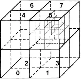
We use an octree to extract the shapes, i.e., distributions of data points in 3D coordinate space, of all members to perform shape-based member comparison and aggregation. An octree [17] is a three dimensional analogy of a quadtree where each node is recursively subdivided into eight children. Subdivision terminates when a stopping condition is reached, for example, when the height of the octree reaches a user defined maximum level. Octrees are widely used for memory reduction in 3D model storage. Figure 4.1 illustrates an octree representation of a 3D mesh model [22].

Figure 4.1: Building an octree to represent a 3D mesh model

Figure 4.2: Octree-based hierarchical spatial subdivision

of all the members in ensemble_Et, the octree construction begins with a root node representing

a minimum bounding cube or octant that covers all data points in the ensemble. We recursively subdivide a parent octant into eight equal-sized, non-intersecting child octants for each member

mi,t (Figure 4.2), until the number of points within the octant is less than or equal to a user

defined upper boundNmaxor the height of octree reaches a user defined maximum depthHmax.

To save memory and reduce compute time, we do not create empty octants that contain no points from anymi,t. Each octant (i.e., octree node) encodes: (1) a pointer to its parent octant;

(2) a key, 0-7, to identify its relative location in the parent octant; (3) coordinates of the octant; (4) a set of pointers to its child octants; (5) the average location, average and variance of data value for each member’s data points.

Several features of the octree representation inspire us to use it in ensemble analysis. An ensemble member normally contains a large number of unorganized data points. For example, static RHIC members contain between 180,000 and 3,300,000 data points. This makes ensemble members expensive to store and render, especially when rotation, translation or animation are involved. Some method to reduce the size of the data is often needed. Existing ensemble visualization algorithms (e.g., pairwise sequential animation [31]) use cluster-based algorithms to select a subset of points that match spatial distributions of attribute values, but they do not correlate sample points from different members and cannot easily perform similarity calculation. An octree representation not only reduces data size by aggregating multiple data points in an octant, but it also links spatially related points from different members by assigning them to the same octant, enabling octant-by-octant shape comparison. Additionally, octrees naturally extract 3D shapes at multiple levels of detail, adding flexibility to the resulting visualization and shape comparison. For instance, a static RHIC member with 700,000 data points is represented by an octree, with_Nmax = 300 containing about 6000 octants.

4.2

Shape Dissimilarity Measurement

The ensemble visualizations described in Section 2.6 rely on humans to intuitively measure differences or correlations between ensemble members. We provide a mathematical measure of pairwise shape dissimilarity between members based on their octree representations. We define the shape of a static member as the distributions of data points in 3D space, and not simply its outer surface position. This shape dissimilarity measure lays a foundation for hierarchical overviews of inter-member relationships. Scientists do not have to predict relationships between members beforehand to decide which subset of members to analyze and visualize.

calculation. Zhang and Smith’s algorithm builds octree representations with a user-specified height for 3D mesh models, labeling each leaf octant as partial or empty. It then compares octants sequentially from each level, with each result scaled and aggregated to produce a final similarity score. Let octrees OA and OB represent 3D objects A and B,S

(l)

i,j be the similarity

score between octant o(_il) in OA and octant oj(l) inOB,o(il) and o

(l)

j both at level l. Zhang and

Smith [50] calculate similarity betweenOA andOB as follows:

SA,B = N

X

i=0

s(_i,il) (4.1)

S(_i,jl) = 1

8l ×ni,j (4.2)

ni,j =

  

1, ifo(_il) ofOA ando(jl) of OB are both labelled partial or empty;

0, otherwise.

(4.3)

The algorithm works well for the shape retrieval problem in [50], but accuracy may not be guaranteed if this approach is applied verbatim to our pairwise member comparison. Instead of building octrees independently for each object, we generate a consistent octree representation whose root octant covers data points from all members of_Et. Given this, it is possible that data

points for some member only distribute in a small sub-region of the root octant. In that case, two members with significantly different shapes may be incorrectly assigned a high similarity because they have numerous empty octants in common. Additionally, to ensure an upper bound of SA,B of 1, each octant in [50] always contains eight children. This may not be true in our

octree since we exclude empty octants.

To support follow-on shape clustering, our system measures dissimilarity between members (as opposed to similarity). We extend Zhang’s algorithm to maintain the accuracy of the dis-similarity calculation for octree representations with large common empty regions. Suppose we want to compare the shapes ofma,t andmb,tinEt. Letdis(il) be the dissimilarity score between

ma,t and mb,t in octant o

(l)

i , and cnt

(l)

a,i and cnt

(l)

b,i be the numbers of data points of ma,t and

mb,t respectively in o(il). The calculation does not compare ma,t and mb,t at any octant that

is empty for both members. It considers ma,t and mb,t as equivalent ato(il) if they have same

point counts, as totally different if o(_il) is empty for either ma,t or mb,t, and partial different

otherwise. We first measure dissimilarity betweenma,t and mb,t at each octant as follows:

dis(_il)=

cnt

(l)

a,i−cnt

(l)

b,i

maxcnt(_a,il), cnt(_b,il)

The range of dis(_il) is [0,1], with a higher score indicating a larger relative difference of point counts between ma,t and mb,t.

Next we aggregate dissimilarity betweenma,tand mb,tat each level. Given levell withN(l)

octants containing points for at least one member, the dissimilarity between ma,t and mb,t at

levell is:

dis(l)=

PN(l)

i=1 dis (l)

i

N(l) (4.5)

Based on Eq. 4.4 the maximum value ofdis(_il) is 1, soN(l) _{is the maximum possible value for}

PN(l)

i=1 dis (l)

i producing a range fordis(l) of [0,1].

Finally, we aggregate dissimilarity measurements from each level, starting at the root, to create a final dissimilarity score. Let H be the height of the octree, and DIS be the final dissimilarity score betweenma,t andmb,t, then

DIS=

PH

l=1w(l)dis(l)

PH

l=1w(l)

(4.6)

A weight factorw(l)_{= 1/r}l_{scales the dissimilarities at different levels in the octree according to}

a shape comparison ratio r, assigning heavier weights to more abstract levels (i.e., levels closer to the root) if 0 < r < 1, lighter weights to more detailed levels (i.e., levels further from the root) ifr >1 and equal weights to all levels ifr= 1. The range ofDISis [0, 1] where DIS= 0 indicates full similarity and DIS= 1 indicates complete dissimilarity.

In practice, we may not always want to compare the octree at all levels. A point number comparison at the root is probably too abstract and a shape comparison at the bottom level may be too detailed. To provide more flexibility in dissimilarity measurements, we enable the dissimilarity calculation to start at a user-specified level Hstart and stop at level Hstop (1 ≤

Hstart ≤ Hstop ≤ H), so that abstract shape information above Hstart and detailed shape

information belowHstop will be ignored.

In conclusion, we alter previous work in [50] in the following ways:

• Each octant is not treated simply as partial or empty, instead, it counts the number of data points of each member in the octant and measures the relative differences.

• The range of a dissimilarity score is [0,1], where 0 represents full similarity, 1 indicates complete dissimilarity, and a higher score implies a higher percentage of differences. • Multiple levels of shape detail are considered. Comparison does not need to happen

throughout the entire octree. Stopping at a level closer to the root omits shape differ-ences at more abstract levels.

comparison ratio, enabling scientists to adjust the shape measure strategy according to their interests.

4.3

Cluster Tree Visualization

The dissimilarity calculations in Section 4.2 produce an N _×N dissimilarity matrix encoding shape dissimilarities between all member pairs in Et. Based on the dissimilarity matrix, we

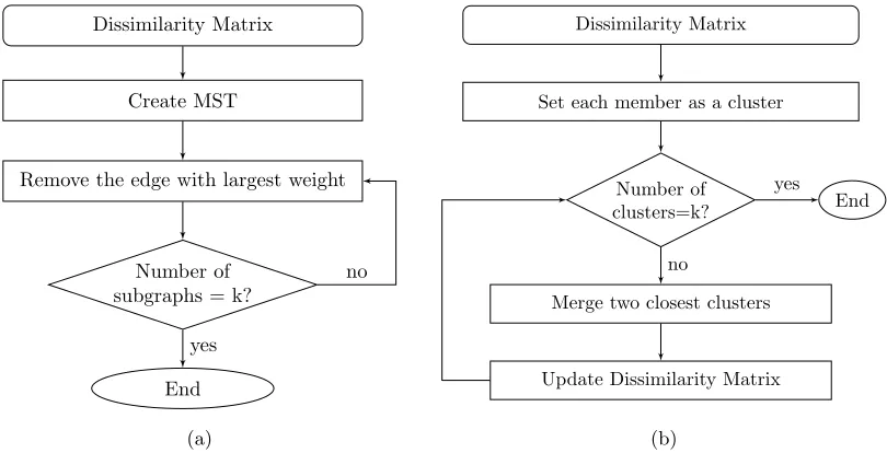
apply two different cluster approaches, a MST based clustering technique and an agglomerative clustering technique, to organize members into groups so that each member is similar to those from its own group and is dissimilar to those belonging to other groups. We visualize the hierarchical clustering results as a cluster tree to provide scientists a better understanding of shape based inter-member relationships in the static ensemble.

Dissimilarity Matrix

Create MST

Remove the edge with largest weight

Number of subgraphs = k?

End

no

yes

(a)

Dissimilarity Matrix

Set each member as a cluster

Number of

clusters=k? End

Merge two closest clusters

Update Dissimilarity Matrix no

yes

(b)

Figure 4.3: Two clustering techniques applied in our system: (a) a top-down MST based clus-tering; (b) a bottom-up agglomerative clustering

4.3.1 MST Based Clustering

Figure 4.4: MST cluster tree showing hierarchical clustering results of 20 members, red nodes highlighting clustering results withk= 7 or σ= 0.21

such as Kruskal or Prim, then recursively removes the edge with the largest weight until the MST has been divided into k subgraphs or until the largest edge exceeds a pre-defined cut-off thresholdσ. Subgraphs of vertices connected by edges belong to a common cluster.

Continuously removing the longest edge until each subgraph contains only one node, we have a series of clustering results assigning members into k= 1 to k=N clusters. We create a cluster tree visualization encoding all the clustering results. Figure 4.4 shows the MST based cluster tree visualization of a 20-member static RHIC ensemble. The cluster tree consists of 39 nodes, each representing a cluster (subgraph) during MST clustering. We assign a unique ID (1 to 39) to each cluster. The ID of a leaf node, i.e., one member cluster, is equivalent to the ID of the member it contains. The opacity of a node is proportional to the number of members the cluster contains. The system enables scientists to control the clustering algorithm by defining a

Figure 4.5: Agglomerative cluster tree visualizes hierarchical clustering results of 20 members, red nodes highlighting the clustering result defined byk= 5 or σ= 0.23

4.3.2 Agglomerative Clustering

Agglomerative clustering (Figure 4.3b) is a bottom-up hierarchical clustering procedure. It starts by assigning each member to a separate cluster, then recursively merges the two most similar clusters and updates the dissimilarity matrix, until all members are assigned into k

clusters or dissimilarity between the two closest clusters exceeds a cut-off threshold σ.

A key procedure in agglomerative clustering is updating the dissimilarity matrix, every time two clusters are merged, to measure the dissimilarity between the new and old clusters. Let s

and t be any members in clusters _A and _B, ds,t be the dissimilarity betweens and t, dA,B be the dissimilarity betweenAandB, and|A|and |B|be the number of members inAand B. We cite three methods to measure dissimilarity between clusters, taken from the Titan Informatics Toolkit [39]:

• Complete-linkage always chooses the maximum dissimilarity between members of each cluster:dA,B=max{ds,t:s∈ A, t∈ B};

• Single-linkagealways chooses the minimum dissimilarity between members of each cluster:

dA,B =min{ds,t:s∈ A, t∈ B};

• Group average linkage calculates the mean dissimilarity between members of each cluster:

dA,B = _|A|·|B|1 P

s∈A

P

t∈B

ds,t .

(a) cluster 17 (b) cluster 31

(c) cluster 32 (d) cluster 34

(e) cluster 35

the other two methods, but its calculation is also more complex.

Applying the clustering procedure until all members belong to one cluster, we have a series of clustering results consisting ofk=N tok= 1 clusters. In contrast to MST based clustering, where the cluster tree is built starting from the root node, agglomerative clustering constructs the cluster tree starting at one-member clusters. We create a cluster tree visualization encoding all the clustering results. Figure 4.5 is the agglomerative cluster tree visualization of the same 20-member RHIC ensemble illustrated in MST clustering. The red nodes highlight the clustering result determined byk= 5 or σ= 0.23. Figure 4.6 visualizes the five clusters in this clustering result.

Agglomerative clustering is more time consuming than MST clustering since it updates the dissimilarity matrix frequently, but it provides clustering results with higher quality be-cause it measures dissimilarity between clusters in each iteration. An agglomerative cluster tree (Figure 4.5) is usually better balanced than a MST cluster tree (Figure 4.4). In practice, we favor the agglomerative clustering technique. The cluster tree visualization provides a high level overview of the hierarchical inter-member relationships and makes it easier to choose a subset of members to comparatively analyze and visualize.

4.4

Visualization

We support two types of glyph-based visualization of _Et based on its octree representation: a

single member visualization and a cluster visualization. The single member visualization displays detailed distributions of shape and attribute value for a single member. The cluster visualization displays summarization and comparison of shapes and attribute value distributions for multiple members.

4.4.1 Single Member Visualization

We use a glyph-based volume rendering technique to display a single static ensemble member

mj,t, each glyph encoding member data in a single octant. Let Pi,j ={p1, p2, ..., pn}be the set

of data points of mj,t in octanto(il). We create a glyphgi foro(il) as follows:

• The location ofgi is the average location of points inPi,j.

• The size ofgi indicates number of points inPi,j.

• The color ofgi represents the average of the attribute values of the points inPi,j.

we can take advantage of the hierarchical structure of an octree to naturally encode shape and data at different levels of detail. An octant from a more abstract level covers a larger 3D space, thus its corresponding glyph should provide a more abstract view of shape and attribute value distributions, possibly preventing the viewer from being distracted by details that are not of interest. This also enables member visualization at different levels of detail without the need to rebuild the octree.

Figure 4.7 visualizes one member at two different levels of detail. Distributions and sizes of glyphs represent volume shape and density of data points. We visualize one attribute at a time. The hue of color scales from blue to red representing the attribute values from small to large. In Figure 4.7, we choose the attribute of temperature to visualize. The hue of color from blue to red represents the temperature from cold to hot. The visualization shows that the member has a cylinder like shape, with a narrowing in the middle. If we cut the cylinder into two parts through the middle, the distributions of data points are sparser in the areas further from the connected region. In both sides of the cylinder, temperature is red (hot) in the middle and gradually reduces to blue (cold) at the boundary. Visualization at a lower level (Figure 4.7a) includes more glyphs and thus presents more details in shape and data distributions.

4.4.2 Cluster Visualization

Visualization of multiple members is one of the key differences between 3D ensemble visualiza-tion and tradivisualiza-tional volume rendering, because ensemble analysis focuses not only on features of a single volume, but also on relationships between members. Ensemble-Vis [34] places mem-bers side-by-side with multiple linked views, assigning the responsibility for comparison to the viewer. Another straight forward solution is to directly render multiple members simultaneously on the screen. This was shown in [31] to be inefficient and prone to on-screen clutter.

To address these issues, we propose a cluster visualization which extends the glyph-based single member visualization to display similarities and differences in shape and attribute distri-butions of multiple ensemble members. The visualization starts with an octant-by-octant data summarization and comparison within the octree, creating a single glyph for each octant and discarding octants that are empty for all members. It then uses the same strategies as those in a single member visualization to select a subset of octants to render (i.e., visualization at multiple levels of detail).

Let _Et0 = _{mk1,t, mk2,t, ..., mks,t},E

0

t ⊆ Et, be a cluster of members to visualize. For any

mkj,t ∈ E

0

t with a non-empty set of points Pi,j in octant o(il), we merge the data of Pi,j into a

new data pointp0_i,j, setting the position and attribute values ofp0_i,j as the average of the points in Pi,j. This produces a list of merged points P

0

i = {p

0

i,k1, p

0

i,k2, ..., p

0

i,ks}, discarding members

with no data ino(_il). The glyphgi ofE

0

t ato

(l)

(a)

(b)

• The location ofgi is the average location of points inP

0

i;

• The color ofgi represents the average attribute value of points inP

0

i;

• The size ofgi represents the number of members inE

0

t for which o

(l)

i is not empty;

• Animation is introduced, with flickering frequency of glyphs fading in and out representing the variance of the attribute values of points in _Pi0.

Figure 4.8e is a cluster visualization of the four members in Figure 4.8a-d. The larger glyphs on the two sides of the dumb bell indicate more members have data in these areas. The smaller glyphs in the central connector between the two sides indicate that the four individual members connect differently. The average temperature of these four members is high in the center of both sides of the dumbbell and decreases gradually toward the boundaries. There are a few points in the center of the two sides that flicker more frequently, indicating higher temperature variances in these octree regions.

(a)

(b) (c)

(d) (e)

Chapter 5

Temporal Ensemble Analysis

The static ensemble analysis in Chapter 4 supports a scalable approach to analyze an ensem-ble at a particular time-step, i.e., a subset of a temporal ensemensem-ble. To analyze relationships between time-series members, we need to consider changes in shape or data value in the time dimension. In this chapter, we extend the static analysis system in Chapter 4 to include anal-ysis and visualization of a temporal ensemble E ={M1, M2, ..., MN}, time-series member Mi,

1 _≤ i_≤ N, consisting of a sequence of T member items (mi,1, mi,2, ..., mi,T). Specifically, the

extended system supports comparison, exploration and visualization of ensembles that respect the contiguous changes in data over time.

The extended system still uses octrees to extract shapes in the ensemble (Section 4.1) (Fig-ure 5.1a), and calculates shape dissimilarity between member items using octree representations (Section 4.2).

To analyze inter-member relationships in ways that highlight the variation of shape over time, we measure similarity between pairs of time-series members. Individual member items are initially clustered into member segments (Figure 5.1b). Amember segment (msi) combines

member items that are similar in shape and located in the same local region in the time dimen-sion. Transforming sequences of member items to sequences of member segments can reduce the length of time-series members and improve performance of pairwise member comparison. The position of different member segments can then be warped based on pairwise segment similarity, using a technique called dynamic time warping (DTW) that aligns shape change between the two members as closely as possible (Figure 5.1c). This allows us to optimize the calculation of pairwise member similarity, which can then be used to construct a hierarchical time-series member cluster tree (Figure 5.1d).

(a)

(b)

(c)

(d)

(a)

(b)

(c)

(d)

(e)