Monte Carlo simulation and Reference Hypernetted Chain equation results for structural, thermodynamic, and dielectric properties of polar heteronuclear diatomic fluids

for structural, thermodynamic, and dielectric properties of polar

heteronuclear diatomic fluids

M. Lombardero and C. Martı´n

Instituto de Quı´mica Fı´sica Rocasolano, CSIC, Serrano 119, E-28006 Madrid, Spain and Departamento de Quı´mica Fı´sica I, U. Complutense, E-28040 Madrid, Spain

E. Lomba

Instituto de Quı´mica Fı´sica Rocasolano, CSIC, Serrano 119, E-28006 Madrid, Spain

F. Lado

Department of Physics, North Carolina State University, Raleigh, North Carolina 27695 ~Received 14 September 1995; accepted 8 November 1995!

We study fluids of heteronuclear two-center Lennard-Jones molecules with embedded point dipoles using both numerical simulation and integral equation theory. Extensive Monte Carlo simulations are performed for the structural, thermodynamic, and dielectric properties of two models of such fluids, with unusually long simulation runs to assure convergence of the dielectric constant. The results are used to test a generalization of a reference hypernetted chain approximation~RHNC-VM! used previously for nonpolar heteronuclear diatomics. Very good agreement is found between the two methods. We conclude that the RHNC-VM integral equation is a reliable method for studying both polar and nonpolar fluids of diatomic molecules. © 1996 American Institute of Physics.

@S0021-9606~96!01507-X#

I. INTRODUCTION

In a recent paper,1we have applied, with good results, a reference hypernetted chain~RHNC!approximation to fluids of uncharged heteronuclear diatomic molecules with site– site Lennard-Jones interactions. This approximation, denoted RHNC-VM, which has proven to be equally successful for homonuclear systems with and without quadrupolar interac-tions~see Ref. 1 and references therein!takes, as a reference system, a fluid of hard diatomics whose atomic diameters, da and db, depend on the temperature T and the densityrof the fluid of interest according to the empirical relation1

d_a5s_ag~g!@252ln~kT/e_a!#@251ln~rs_a3!#, a5a,b

~1!

with

g~g!5a

F

S

D

2

G

where g5s_b/s_a<1, e_a, s_a being the Lennard-Jones pa-rameters for the aa atomic interactions, and in Eq. ~2!

a51.6231023 and h50.98 ~Ref. 2! are adjustable param-eters. Their values have been determined by requiring that, for some convenient thermodynamic state at high density, the computed values of the principal thermodynamic quanti-ties should reproduce known Monte Carlo results.1 In the spirit of the Rosenfeld–Ashcroft3 universality principle, these values are then taken to be essentially unchanging for all potentials of the same symmetry; a similar treatment is made for the parameter m introduced later in Eq.~3!. In the RHNC-VM closure relation, the reference system bridge function B0(12) is then constructed with these diameters

us-ing an approximation formulated for hard spheres by Verlet4 some years ago and later modified for homonuclear and het-eronuclear hard diatomics by Labı´k et al.5

In the present work, continuing a progression towards more complex models that might consistently describe real fluids, we consider a dipolar fluid composed of heteronuclear diatomics with Lennard-Jones interatomic potentials and a point dipole at the molecular center of mass ~2CLJD!. In order to build directly into the reference system the molecu-lar asymmetry introduced by the dipole, we reformulate the previous expression for the atomic diameters to explicitly incorporate the dipole momentm, now putting

d_a5s_ag~g!

S

ea~12mm2/easa3!

D

3@251ln~rs3_a!#, a5a,b ~3!

where, as in Eq. ~1!,g5sb/sa<1. We complete the speci-fication of the reference model by assigning to it the same molecular elongation as the ‘‘real’’ fluid, so that LHD/da5L/sa5L*, where LHD and L are the respective distances between atomic centers in the two systems.

The g(g) function, and more specifically the parameter h, reflects the differences in atomic diameters, while the pa-rameter m, also adjustable, is associated with the dipole mo-ment. We note that Eq.~3!is constructed so that ifm50 and

sa5sb ~g51! the resulting theory is that of a nonpolar homonuclear fluid.6

dipolar. In the present study these are separately and explic-itly accounted for in the reference model through Eq. ~3!, while in the earlier work they are implicitly introduced through a single adjustable parameter,g, whereby d_b5gd_a, where

d_a5as_a@252ln~kT/e_a!#@251ln~rs_a3!#.

The fundamental relations of the theory of liquids are the Ornstein–Zernike ~OZ! equation coupling the indirect and direct correlation functions, g~12!and c(12),

g~12!5 r

4p

E

and the closure relation which, in the RHNC-VM approxi-mation, is written as

c~12!5exp@2bu~12!1g~12!2B0~12!#2g~12!21, ~5!

whereb51/kBT, u(12) is the intermolecular potential, and B0(12) is the bridge function of the reference system

de-scribed earlier. With the exception of Eq.~3!, which replaces Eq.~8!of Ref. 1, further details on the use of the RHNC-VM approximation are as described in that earlier work on non-polar heteronuclear systems, to which the reader is referred. For completeness, we have also carried out systematic Monte Carlo ~MC!simulations for the structural, thermody-namic, and dielectric properties of the models considered here. There appear to be in the literature no additional simu-lation studies for heteronuclear 2CLJD systems beyond the molecular dynamics calculations of Murad et al.8for hydro-gen chloride and the MC calculations carried out by us7,9for the same system. Even for the simpler case of homonuclear 2CLJD models, available results known to us are limited to those of Fisher and co-workers10,11for the refrigerant R152a

~CH₃–CHF₂!, modeled as a fluid of this type.

The most significant electrostatic property of a material system is doubtless its dielectric constant, which measures the response of the system to an external electric field. It is however also the most problematical for computer simula-tion, in part due to the very long runs needed to obtain reli-able values of this slowly-converging quantity. This may be one of the reasons for the scarcity of such data, especially for ‘‘realistic’’ models like those considered here. To help alle-viate this deficiency, we have carried out high-precision, sys-tematic simulations for the dielectric constant of our models, with runs of up to 4503106configurations~depending on the thermodynamic conditions! to guarantee the stability of the computed values.

II. POTENTIAL MODEL AND PARAMETER m

The intermolecular potential u(12) of a heteronuclear 2CLJD system with the~ideal!molecular dipole aligned with the molecular axis is given by

u~Rv1v2!5u2CLJ~Rv1v2!1uDD~Rv1v2!. ~6!

The first term in this expression is the two-center Lennard-Jones ~2CLJ!potential

u_2CLJ~Rv₁v₂!5

(

ab uab~r!, a,b5a,b, ~7!

where

u_ab~r!54e_ab

FS

D

12

2

S

D

6

G

is the interaction between atomsaandbof molecules 1 and 2, respectively, separated by a distance r5r(Rv1v2). In

these expressions, R5uR22R1u is the separation between

molecular centers with positions R1, R2andv1,v2 are the

molecular orientations. For simplicity, we will write the Lennard-Jones parameterse_aa,e_bb,s_aa, ands_bbase_a,e_b,

sa, andsb. The parameterseab5eba andsab5sba associ-ated with the cross interactions are defined by the usual mix-ture rules,

eab5~eaeb!1/2, ~9!

sab512~sa1sb!. ~10! The second term of Eq.~6!is the dipole–dipole interaction,

uDD~Rv1v2!52

m2

R3 @3~n•s1!~n•s2!2s1•s2#, ~11!

where n is a unit vector in the direction of R5R₂2R₁ and s1, s2are unit vectors in the directions of the dipole moments

of molecules 1 and 2, respectively.

The dipole–dipole interaction is notably long-ranged for computer simulations. To account for the long-range contri-butions we have adopted the reaction field ~RF!method,12,13 which appears to be the most advantageous for establishing direct comparisons between theory and simulation.14 In this approximation scheme, the interaction potential u(12) is truncated at a distance Rc, the cutoff radius, determined es-sentially by the size of the simulation cell. A given dipole i of the sample interacts with its neighbors within the sphere of radius Rc~centered on the dipole!according to the dipolar potential ~11!and with the remainder, treated as an infinite, continuous, and polarizable dielectric medium of dielectric constante_RF, through a mean reaction field15,16

Ri5

2~e_RF21!

~2eRF11! M_i

R_c3, ~12!

generated at the position of dipole i by the polarization of the dielectric due to the total dipole moment M_iof the truncation sphere about i.

Neumann and Steinhauser15 have shown that the RF method is equivalent to using an effective potential given by13,15

ue~12!5

H

u~12!1uRF~12! R,Rc

0 R.Rc,

~13!

where uRF~12!is the contribution of the interaction with the

reaction field,

uRF~12!52

2~eRF21! ~2eRF11)

m2

To make theory and simulation directly comparable,14 all results in both methods have been obtained using the effec-tive potential ue(12), with the same values of the parameters RcandeRF, rather than the original potential u(12) given by

Eqs.~6!–~11!. The cutoff radius has been determined accord-ing to the standard relation Rc5

1 2(N/r)

1/3

, where N is the number of molecules in the simulation sample.

We summarize in Table I the molecular parameters of the two ~arbitrary! models, A and B, for which we have carried out calculations. ~In the table, t5Pb/ Pa is the ratio of atomic weights.!Most of the study focuses on model A, which has been chosen for theoretical consistency in fixing m ~see the following!; it corresponds to the model of a non-polar heteronuclear fluid used in Ref. 1 to determine the value of the parameter h associated with the difference in atomic sizes. Although it is an arbitrary model, its Lennard-Jones parameters,e_aands_a, match those of a nonpolar sys-tem considered by Murad et al.8as a model of liquid HCl in molecular dynamics studies.

Model B differs from model A only in having a smaller molecular anisotropy (L*50.2), all other parameters being the same. This model is included in our study to accentuate the effects of the dipolar anisotropy over those of the geo-metric one, thereby permitting a stricter test of the capacity of the theoretical construction to deal specifically with the dipole–dipole interaction. The molecular geometries of the two models are contrasted in Fig. 1.

The reference system parameter m of Eq.~3!remains to be fixed to complete the theoretical scheme of the RHNC-VM approximation. As with the other two param-eters~aand h!of Eq.~3! ~see Ref. 1 and references therein!, m has been determined by requiring that, at a given tempera-ture and density, the theoretical results for the

compressibil-ity factor and internal energy simultaneously match as closely as possible those of simulation. As noted earlier, we make the underlying assumption that these parameters are ‘‘universal’’ in that values determined for a particular mo-lecular model should be equally valid for at least all other potentials of the same symmetry group. Thus, the new pa-rameter m has been adjusted while maintaining the previous values ofaand h obtained form50.

For reasons of consistency, we have chosen m using the same molecular model as in Ref. 1 for the parameter h, to which we have simply added a reduced dipole moment

m*2_[m2_/e

asa

3_{51.50, which corresponds to the dipole}

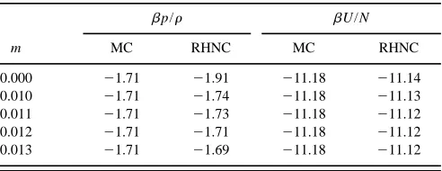
mo-mentm51.422D of Table I. The adjustment was carried out in both cases for the same state point, T*50.8 andr*50.75, lying in a region of low temperature and high density. In Table II we compare with MC the theoretical values of the compressibility factor and internal energy for different m, choosing

m51.231022 ~15!

as the universal value for all calculations.

Table II also includes the value m50. In this case the resultant expression for d_a is the one previously determined for a nonpolar heteronuclear fluid in Ref. 1, Eq. ~1!. The extent of the discrepancy seen here for the compressibility factor demonstrates the need for introducing the new param-eter m in extending the theory to polar systems.

III. STRUCTURE AND THERMODYNAMICS

In this section and in Sec. IV we compare theory with simulation. To facilitate that comparison, following Patey et al.,13we have computed all results in both cases using the effective potential ue(12), given by Eqs.~13!and~14!, rather than the original potential u(12).

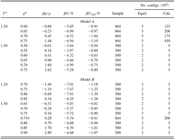
For the numerical work, we have chosen the same re-duced temperatures~T*51.20 and 1.50!and reduced dipole moment ~m*2_{51.50!for both model A and model B. Since}

the two models also share the same Lennard-Jones param-eterse_aands_a ~Table I!, this implies identical physical val-ues of temperature T and dipole momentmin the two cases. Table III gives the MC results for the compressibility factor bp/r, the internal energy bU/N, and the dipole– dipole contribution to the energybU_DD/N, for models A and B of Table I. In the simulations, we have applied different criteria for cases that did or did not include the dielectric constant. For the latter cases we have worked with 500 mol-TABLE I. Molecular parameters for the model fluids included in this work.

Parameter Model A Model B

ea/k 259.0 K 259.0 K

eb/k 20.0 K 20.0 K

sa 3.353 Å 3.353 Å

sb 2.735 Å 2.735 Å

m 1.422 D 1.422 D

L 1.257 Å 0.671 Å

t 0.0284 0.0284

FIG. 1. Molecular geometries of models A and B.

TABLE II. Theoretical compressibility factor and internal energy vs MC

data at T*50.8,r*50.75, and several m values for model A of Table I.

m

bp/r bU/N

MC RHNC MC RHNC

0.000 21.71 21.91 211.18 211.14

0.010 21.71 21.74 211.18 211.13

0.011 21.71 21.73 211.18 211.12

0.012 21.71 21.71 211.18 211.12

ecules and runs of 23106 configurations for equilibration and 53106more for data taking, while for the former cases we have used samples of 864 molecules with data-taking runs of 1253106 to 4503106 configurations following 53106of equilibration. Throughout this study we have used

eRF57.20 for the dielectric constant of the continuous

me-dium, a value of the order of magnitude suggested by earlier exploratory runs.

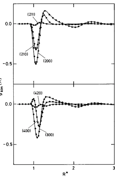
Theory and simulation are graphically compared in Figs. 2– 8. For the structural properties, we have chosen as repre-sentative the results from the state point T*51.20,r*50.70 for model A and T*₅1.20,r*₅0.80 for model B. In Fig. 2 we show the center-to-center distribution function g000 @

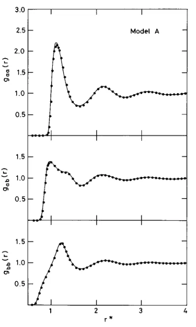
ra-dial component of the molecular distribution function g(12)# and in Fig. 3 the first three angular components gklm of g(12) in the axial frame of reference. In Figs. 2 and 3 the upper part corresponds to model A and the lower to model B. Figure 4 shows a few higher-order angular components for model A but not for model B. The latter case approximates a Stockmayer fluid~see Fig. 1!with components gklmfor k.1 that are almost inappreciable on the scale of Fig. 4. Finally, in Figs. 5 and 6 we show the theoretical curves obtained for the three different atom–atom pair distribution functions g_ab(r) for both models A and B, respectively, contrasted with the corresponding MC points. The theoretical curves are obtained by direct integration over the molecular pair distri-bution function g(12) following the method recently de-scribed in Ref. 17.

The theoretical results~solid line!and simulation~solid circles! for the thermodynamic properties are jointly pre-sented in Fig. 7 for model A and in Fig. 8 for model B. From

TABLE III. Compressibility factor and internal energies from MC simulation.

T* _r* bp/r bU/N bUDD/N Sample

No. configs.~106!

Equil. Calc.

Model A

1.20 0.60 20.60 25.65 20.91 864 5 125

0.65 20.23 26.09 20.97 864 5 200

0.70 0.45 26.52 21.04 864 5 175

0.75 1.48 26.94 21.10 864 5 450

1.50 0.50 20.01 23.64 20.56 500 2 5

0.55 0.16 23.97 20.60 500 2 5

0.60 0.41 24.32 20.65 500 2 5

0.65 0.90 24.66 20.70 500 2 5

0.70 1.60 24.99 20.75 500 2 5

0.75 2.62 25.28 20.80 500 2 5

Model B

1.20 0.70 21.49 27.01 21.18 500 2 5

0.75 21.19 27.47 21.25 500 2 5

0.80 20.60 27.91 21.30 500 2 5

0.85 0.34 28.35 21.38 500 2 5

1.50 0.65 20.51 25.03 20.81 500 2 5

0.70 20.28 25.37 20.85 500 2 5

0.75 0.16 25.72 20.90 500 2 5

0.754 0.20 25.76 20.91 864 5 200

0.80 0.79 26.08 20.96 500 2 5

0.85 1.70 26.39 21.01 500 2 5

0.90 2.89 26.68 21.07 500 2 5

FIG. 2. Center-to-center distribution function g000(R) for model A at

T*₅1.20 andr*₅0.70 and for model B at T*₅1.20 andr*₅0.80. Solid

top to bottom these figures show~a!the compressibility fac-torbp/r,~b!the internal energybU/N, and~c!the dipole-dipole contribution to the energy bUDD/N.

Direct inspection of all these figures shows that the agreement between theory and simulation is quite good, for both the structural~Figs. 2–6!as well as the thermodynamic

~Figs. 7 and 8!properties. The level of agreement between the two techniques is furthermore similar for both model A and model B.

The novelty of the RHNC-VM approximation we are examining lies in its generalization to include dipolar forces through an empirical relation between the geometry of the reference system and the dipole momentmof the system of interest. Since the thermodynamic property most directly coupled to these forces is the dipole–dipole contribution to the energy, bUDD/N, this quantity is particularly useful in checking the theory. In the Figs. 7~c!and 8~c!we see that the theoretical values lie systematically slightly above those of simulation, an apparent theoretical overestimation. Their relative deviations from the MC points, however, are every-where less than 3%; given the small magnitude of this quan-tity, the theoretical predictions may be taken as completely satisfactory. This is particularly significant for model B, since the small elongation of this case accentuates the dipolar effects compared to those of the structural anisotropy.

IV. DIELECTRIC CONSTANT

The strong dependence on long-range forces of the di-electric constant emakes its calculation by computer

simu-lation, as well as comparisons between simulation and theory, problematical topics even today. Presentation of re-sults of this nature must therefore carefully specify both the conditions of the simulation as well as the chosen procedure for properly comparing the two sets of results, theoretical and simulated.

For fluids of polar, nonpolarizable molecules, use of the RF boundary conditions leads to anesatisfying13,18

~e21!~2eRF11!

3~2e_RF1e! 5y g, ~16!

where y54pbrm2/9 and g is the Kirkwood factor. The computation of g obviously will differ in the two ap-proaches, simulation and theory.

If N is the number of identical molecules in the cubic simulation cell and M5Smk(k51,...,N) is the total dipole moment of the cell, the g factor is found from the mean square moment ^M2&according to13,19,20

g5

^

2

_&

Nm2, ~17!

wherem5um_ku. Equations~16!and~17!jointly constitute the fluctuation formula for the dielectric constant e to be used when, as here, RF boundary conditions are adopted in the simulation to correct for the long-range effects. It should be noted that this procedure implies that ^M&50; thus, as a simulation proceeds, fluctuations in M should evolve such FIG. 3. First angular projections of the molecular distribution function

g(12) in the axial reference frame for model A at T*₅1.20 andr*₅0.70

and for Model B at T*₅1.20 andr*₅0.80. Symbols are as in Fig. 2.

FIG. 4. Higher order angular projections of the molecular distribution

func-tion g(12) in the axial reference frame for model A at T*51.20 and

that~^M2&2^M&2!/Nm2→^M2&/Nm2, a condition that must be met, within some specified margin of error, for reliable re-sults.

When, as here, theoretical results for the dielectric con-stant of polar fluids are to be contrasted with those of simu-lation, the original Kirkwood formula21 for infinite systems is no longer valid. Patey et al.13 have shown that for com-parison with simulations using RF boundary conditions, the g factor is to be obtained instead from

g5114pr 3

E

`

h_D~e!~R!R2dR, ~18!

with e again found using Eq. ~16!. In this expression, we have put h_D(e)(R)5h110

(e)

(R)22h111 (e)

(R), where h110 (e)

and h111 (e)

are spherical harmonic coefficients of the total pair correla-tion funccorrela-tion h(e)(12) in an axial frame where the z axis coincides with the molecular axis. The superscript ‘e’ means that while the system is still infinite, the molecular interac-tions occur through the effective potential u_e(12) defined by Eqs. ~13!and~14!rather than the original potential u(12).

Equation~18!can be written equivalently as

g5111 3 r˜h~D

e!_{~0!, ~19!}

where h˜_D(e)(0) is the Fourier transform of h_D(e)(R) for k50. Since h˜_D(e)(k) is computed in the process of solving the OZ integral equation, this latter form minimizes computational error and is to be preferred.

All results forepresented here have been obtained using Eqs.~16!and~17!for MC simulation and Eqs.~16!and~19! for theory. The effective potential ue(12) has been used throughout, with a cutoff radius of Rc5

1 2(864/r)

1/3

deter-mined by the N5864 particles in the MC simulations. These procedures should guarantee, in accord with the findings of Patey et al.,13 that the two sets of values for e may be di-rectly compared.

The achievement of a high level of rigor and reliability in the simulations, within the inevitable limits imposed by available resources, has been a constant concern in this work. This has been particularly true in the calculation of e, for which, given its slow rate of convergence, runs of up to 4503106 configurations have been carried out. The cost in machine time that this entails has meant that simulations have focused primarily on model A, for which four density states have been simulated on the ~low temperature! T*51.20 isotherm, a presumed good sampling of the liquid phase at this temperature. The dielectric constant for model B has been simulated for just a single state, T*51.50 and

r*50.754. This state has been chosen so that the density

FIG. 5. Atom–atom pair distribution functions gab(r) for model A at

rd* 5 rd

3_{, @where d is the diameter of a sphere whose}

vol-ume equals that of a hard diatomic molecule defined by the respective Lennard-Jones parameters s_a ~Ref. 1!# for this state of B matches that of r*50.65 for A. Even if for just one state, the model B calculation is of interest in that it tests the theory on a model different from that used to adjust the RHNC-VM reference system ~see Sec. II!. Since model B additionally gives greater relative weight to the dipolar mo-lecular asymmetry over the geometric, a comparison of the dielectric constants for this case is clearly an important test of the accuracy of the theory.

Table IV summarizes the MC results and includes the number of configurations generated for equilibration and cal-culation for each state. The evolution of e with number of configurations is shown in Figs. 9 and 10 for model A and model B fluids, respectively, while Fig. 11 shows the evolu-tion of the convergence condition ~^M2&2^M&2!/Nm2

→^M2&/Nm2during the course of the simulation for the state T*51.20, r*50.70 of model A. Other states simulated all display a degree of convergence equal to or better than that of Fig. 11 and are not shown.

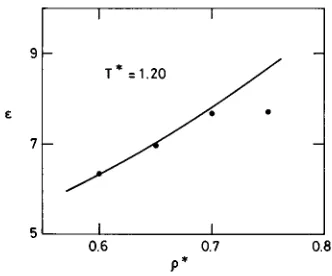
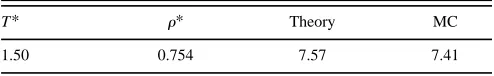
Theoretical results for e are compared to those of MC simulation in Fig. 12 for model A and in Table V for model B. The first notable feature of the figure is the abnormally low value of the simulation result at the highest density,

r*50.75. Assuming no shortcomings in the simulation, dif-ferent explanations may be put forward for this behavior. At

these high densities, for one, we could be seeing the effect of density dielectric saturation due to the competition between short-range packing effects arising from the molecular an-isotropy ~form factor!, on the one hand, and long-range di-electric effects, on the other. The predominance of the first of these over the second would reduce the capacity of the sys-tem to polarize in an external electric field, attenuating ~or even inverting!the rate of growth ofewithr*. If this view is correct, the theory is clearly failing, since it shows no ten-dency for e to saturate. To test whether the phenomenon might show up at higher densities, we have continued the

FIG. 7. ~a!Compressibility factor,~b!internal energy, and~c!dipole–dipole

contribution to the internal energy for model A, as functions of density. Dots and lines stand for MC and theoretical results, respectively.

FIG. 8. ~a!Compressibility factor,~b!internal energy, and~c!dipole–dipole

contribution to the internal energy for model B, as functions of density. Dots and lines stand for MC and theoretical results, respectively.

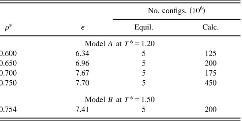
TABLE IV. Dielectric constant from MC simulation of 864-particle samples at several densities.

r* e

No. configs.~106_!

Equil. Calc.

Model A at T*51.20

0.600 6.34 5 125

0.650 6.96 5 200

0.700 7.67 5 175

0.750 7.70 5 450

Model B at T*₅1.50

theoretical solutions ~not shown in Fig. 12! to a density of

r*50.90, with no change in the nature of the theoretical curve. However, we note that some time ago, Nichols and Calef22found that an RHNC scheme could produce dielectric saturation at sufficiently high densities. They suggest that this result, obtained for a model of hard linear triatomics with a hard sphere fluid as reference system, might result from an excessively large diameter of the reference hard spheres. This idea could not be pursued in the present calcu-lation, which uses a different reference system.

An alternative explanation could be that the low value of the simulated eat high densities is an artifact of an

insuffi-cient simulation sample size ~864 particles!, whereby long-range behavior that strongly affects ecannot adequately be reproduced at sufficiently high densities. In such circum-stances, the small sample size and correspondingly small cut-off radius R_c would no longer guarantee the equivalence conditions between theory and simulation implied by Eqs.

~16!–~18!.

In contrast with the discrepancy between theory and ex-periment at high densities, the results for ein a broad range of normal densities covered in the study of model A~Fig. 12! can be characterized as very good. This is also true for the single state of model B, as seen in Table V. Given the deli-cacy and complexity of calculations for the dielectric con-stant, both theoretical and simulated, this must be counted as a notable success for the RHNC-VM theory.

V. DISCUSSION

We have carried out extensive Monte Carlo simulations for two models of fluids of dipolar heteronuclear two-center Lennard-Jones molecules using reaction field boundary con-ditions. The study included structural, thermodynamic, and dielectric properties and their variation with density along two different isotherms for each model. A primary goal of this work has been to furnish simulation data of high preci-FIG. 9. Convergence of the MC dielectric constant along simulation runs.

Results for model A corresponding to the four state points of Table IV

(T*51.20).

FIG. 10. Convergence of the MC dielectric constant along the simulation

run. Results for model B at T*₅1.50.

FIG. 11. Evolution of the fluctuation~^M2_&2^M&2_!/Nm2_{and of the average}

^M2&/Nm2along the simulation run of model A at the state point T*51.20

andr*₅0.70.

FIG. 12. Dielectric constant as a function of density for model A at

T*₅1.20. The solid line represents theoretical results and solid circles stand

sion for this class of fluids, towards which special efforts have been made to assure the best possible conditions of sample size, length of runs, etc., especially for the dielectric constant.

We have also studied in this work an RHNC integral equation approximation which generalizes to this class of fluids a closure relation recently formulated for nonpolar flu-ids with excellent results. The reference system in this ap-proximation is a fluid of hard heteronuclear diatomics whose atomic diameters depend empirically on the temperature and density of the system of interest and in the present version also on its molecular dipole moment m.

A comparison of the theoretical results with those from simulation completes this work: we find a high degree of agreement between the two, not only for the structural and thermodynamic properties but also for the more sensitive dielectric constant. The only significant discrepancy shows up for just this latter property at very high densities. We have no definitive explanation for this disagreement, which may arise from dielectric saturation or ~what seems to us more likely! insufficient sample size at these high densities to properly account for long-range effects due to the dipolar potential.

The overall good results obtained from the theory for the set of properties and dipolar fluid models examined here con-firms and extends the excellent behavior of the RHNC-VM approximation that was already established in earlier studies of the three possible types of nonpolar diatomic fluids

~homonuclear diatomics, quadrupolar homonuclear diatom-ics, and nonpolar heteronuclear diatomics!, in a region of the phase diagram that in each case covers the presumably es-sential part of the liquid state ~see Ref. 1 and references therein!. We may thus conclude in a general sense that this RHNC scheme, based on a closure relation we have denoted RHNC-VM, is a good approximation for diatomic fluids, po-lar and nonpopo-lar. This further supports the assumed univer-sality of the parametersa, h, and m that determine the ref-erence atomic diameters d_a, in the sense that they are essentially unchanging for all potentials of the same symme-try group, reflecting thereby the universality of the reference bridge function.

ACKNOWLEDGMENTS

We thank the Centro Te´cnico de Informa´tica del CSIC and especially the Centro de Supercomputacio´n de Galicia

~CESGA!for generous access to their computing facilities. This work was financially supported by the Spanish Direc-cio´n General de InvestigaDirec-cio´n Cientı´fica y Te´nica~DGICYT! under Grant No. PB94-0112.

1_{M. Lombardero, C. Martı´n, and E. Lomba, Mol. Phys. 81, 1313~1994!.}

2_{It should be noted that this value of the parameter h differs from the value}

used in Ref. 1, h50.89. This difference occurs because in solving the OZ

equation in the earlier work we assumed for greater numerical efficiency a

minimum distance rm*5 0.7 such that uab(r)5` for r* <rm*. In the

present work this unneeded condition has been dropped, thereby changing the calculated value of h to 0.98, as cited and used in this paper. We have also recalculated with this new value of h all theoretical results of Ref. 1. We find that the final results are scarcely affected by the change, save for those instances where appreciable differences existed between theory and

simulation@as in the compressibility factor~Fig. 5 of Ref. 1!or the

spheri-cal harmonic coefficients gk10~Fig. 4 of Ref. 1!of fluid B#, which are now

diminished in good measure. Thus, for example, the compressibility factor

for the thermodynamic state with greatest error, T*₅1.0,r*₅0.75~Fig. 5

of Ref. 1!goes from a value of 1.02 to a corrected value of 0.87,

com-pared with the MC value of 0.64. The discrepancies affecting the gk10

functions are practically eliminated, so that the theoretical curves now

show the same good agreement with the MC results as do the other gklm

coefficients~see Figs. 1–4 of Ref. 1!. The latter good agreement remains.

3_{Y. Rosenfeld and N. W. Ashcroft, Phys. Rev. A 20, 1208~1979!.}

4

L. Verlet, Mol. Phys. 41, 183~1980!.

5

S. Labı´k, A. Malijevsky´, and W. R. Smith, Mol. Phys. 73, 87~1991!; 73,

495~1991!.

6_{M. Lombardero, C. Martı´n, and E. Lomba, J. Chem. Phys. 97, 2724}

~1992!. 7

E. Lomba, C. Martı´n, M. Lombardero, F. Lado, and J. S. Høye, J. Chem.

Phys. 100, 1599~1994!.

8_{S. Murad, K. E. Gubbins, and J. G. Powles, Mol. Phys. 40, 253~1980!.}

9_{E. Lomba, A. Ferna´ndez, C. Martı´n, and M. Lombardero, Phys. Scr. T38,}

79~1991!.

10

C. Vega, B. Saager, and J. Fischer, Mol. Phys. 68, 1079~1989!.

11_{B. Saager, J. Fischer, and M. Neumann, Mol. Simul. 6, 27~1991!.}

12_{J. A. Barker and R. O. Watts, Chem. Phys. Lett. 3, 144~1969!; Mol. Phys.}

26, 789~1973!. 13

G. N. Patey, D. Levesque, and J. J. Weis, Mol. Phys. 45, 733~1982!.

14_{J. M. Caillol, D. Levesque, and J. J. Weis, Mol. Phys. 44, 733~1981!.}

15_{M. Neumann and O. Steinhauser, Mol. Phys. 39, 437~1980!.}

16_{J. A. Barker, Mol. Phys. 83, 1057~1994!.}

17_{M. Alvarez, E. Lomba, C. Martı´n, and M. Lombardero, J. Chem. Phys.}

103, 3680~1995!.

18_{M. Newmann, Mol. Phys. 50, 841~1983!.}

19_{S. W. Leeuw, J. W. Perram, and E. R. Smith, Annu. Rev. Phys. Chem. 37,}

245~1986!.

20

P. G. Kusalik, Mol. Phys. 81, 199~1994!.

21

J.-P. Hansen and I. R. McDonald, Theory of Simple Liquids~Academic,

London, 1986!.

22_{A. L. Nichols III and D. F. Calef, Mol. Phys. 71, 269~1990!.}

TABLE V. Theoretical and MC dielectric constantefor model B.

T* r* Theory MC