Testing Dynamic Models of Worker Effort

of Worker Effort

Stephen Machin,

Alan Manning,

This article derives three dynamic models of worker effort determi- nation, based on a shirking efficiency wage model, a compensating differentials model, and a union-firm bargaining model. It shows that all of these three models have the same long-run comparative statics but differ in their short-run dynamics. We use these different predic- tions about the dynamics as a basis for testing the models. Euler equa- tions for each model are estimated using panel data on 486 U.K. com- panies. The evidence supports the shirking model in firms with low levels of unionization but the bargaining model in highly unionized industries.

I. Introduction

Efficiency wage theories have, in recent years, deservedly attracted a lot of attention as a potential explanation of involuntary unemployment and other aspects of the labor market. However, virtually all the research in efficiency wage theory has been theoretical, and testing the theory has proved remarkably difficult.

One empirical approach (e.g., Krueger and Summers 1988) is to argue that observed interindustry wage differentials are not consistent with com-

We would like to thank seminar participants at Trinity College, Dublin, the Universities of Manchester, Marseille, Warwick, and Bristol, the Institute for In- ternational Economic Studies at the University of Stockholm, and Employment Market Research Unit (EMRU) for their helpful comments. Thanks also go to Xeni Dassiou and John van Reenen for help with setting up the data. Alan Manning would like to thank the Leverhulme Trust for financial support.

[Journal of Labor Economics, 1992, vol. 1O, no. 3]

(? 1992 by The University of Chicago. All rights reserved. 0734-306X/92/1003-0005$01.50

petitive theory but are consistent with some version of efficiency wage theory. However, this evidence is not uncontroversial (e.g., see Murphy and Topel 1987; Gibbons and Katz 1989) and is at best indirect as efficiency wage models are not the only alternatives to competitive theories. Given this, the more direct approach of Wadhwani and Wall (in press) and the "cost-of-job-loss" literature (see, e.g., Weisskopf, Bowles, and Gordon 1983) is refreshing. They argue that the popular shirking version of effi- ciency wage theory (Shapiro and Stiglitz 1984) predicts that worker pro- ductivity is higher the higher are wages in a given firm relative to the utility that workers could get elsewhere. They estimate production functions and find evidence in line with this view. However, as Wadhwani and Wall acknowledge, this finding remains consistent with notions of compensating differentials and with bargaining theory, so the results cannot be interpreted as strongly in favor of efficiency wage theory.

The purpose of this article is to shed further light on these issues. We present dynamic versions of Shapiro and Stiglitz's (1984) shirking model, of a compensating differentials model, and of a bargaining model. We confirm that, in the long run, all models predict that worker effort in a firm will be related to the difference between wages and utility available on the more general labor market. However, the dynamics of effort de- termination are different in the three models. The basis for our test is that, in shirking efficiency wage models, worker effort should be positively related not just to current wages but also to future expected wages, because if wages are going to be high in the future, the cost of losing a job today will be high. As we shall see, the other models do not necessarily have this prediction. This means that if we estimate Euler equations for worker effort we might hope to provide a more discriminating test of efficiency wage theory than has been done before. This is the main advantage of our approach.

However, our approach does have its disadvantages. First, it concentrates on a particular version of efficiency wage theory, namely, the shirking model. Also, the approach puts considerable weight on some dynamic assumptions that may be quite strong. For example, our approach could not really be expected to be a test of the more "sociological" versions of efficiency wage theory (e.g., Akerlof 1982), as it is not clear what a dynamic version of such a model would look like. In addition, our Euler equations are based on Markov perfect equilibria and may not capture the repeated game aspects of efficiency wage models that have been emphasized by Macleod and Malcomson (1989).' For these reasons, we prefer to think

l It would be nice to present a test of the efficiency wage models of Macleod

of the tests presented here as supplementary evidence on the plausibility and importance of efficiency wage theory.

The plan of this article is as follows. In the next section, we present our basic theoretical models: a dynamic shirking model, a compensating dif- ferentials model, and a dynamic bargaining model. In the third section, we discuss how we can base empirical tests on these models. In the fourth section, we implement these tests on a panel of British companies. The results for the overall sample are not consistent with the efficiency wage model and appear to be more in line with the bargaining model than with the compensating differentials model. But, when we split the sample of firms into low and high union industries, the efficiency wage model seems to perform best for the low union sector and the bargaining model seems to perform best in the high union sector.

II. The Theoretical Model

In this section, we present dynamic versions of a Shapiro-Stiglitz model, a compensating differentials (competitive) model, and a bargaining model. The setup common to all three is the following. Assume that workers in a firm at date t get current utility U(W,,e,), where W, is the real wage and et is effort. We assume that Uw > 0, U, < 0. In the empirical section below, to help with the derivation of estimable equations, it will be con- venient to assume that U(W,, et) = wt - et, where lowercase letters denote logarithms. Most of the existing literature makes this assumption that Uw,

= 0, and, as we shall see in the theoretical section, it does make the com- parative statics of the model more clear-cut than they would be otherwise. We assume that there is a probability q that the worker will leave the firm before next year. Then, if we denote the value of a job in this firm in year t by Vt and the value of being on the open labor market by Vt, we will have

Vt = U(Wt, et) + 6[(1 - _{q)EtVt+l + qEtVt+l], (1)}

where 6 is the discount factor and q is the labor turnover rate (which we treat as exogenous). If a worker is on the open labor market, we will assume that his or her current expected utility is zt, which will be deter- mined by wages in other firms, the level of unemployment benefit, and the chance of employment. If we assume that the firm under consideration is small in relation to the rest of the economy, so that a worker never expects to return to the same firm once he or she has left it, we will have2

2 _{One might also want to distinguish two alternative states: employment else-}

where and unemployment. Doing this does not alter the basic prediction of the shirking model that effort should be positively correlated with future wages, but it does introduce an extra set of lags into the estimable Euler equations that are

Vt = '-t + 8EtVt+?. (2)

Using (2), we can write (1) as

(Vt - _{Vt) = U(Wt, et)} - _'it + 6(1 - _{q)Et(Vt+- Vt+l).} (3)

In what follows, we look at Markov perfect equilibria in which the employer cannot commit future wages in advance. So, Vt+1 will be regarded as independent of any decisions taken at time t. This assumption is probably reasonable given that we will be working with annual data and wage con- tracts that are generally 1 year in length in the United Kingdom.

Now consider how we can use these models to analyze the implications of three different labor market models.

A. A Dynamic Shirking Model

Consider the following simple dynamic version of the Shapiro-Stiglitz (1984) model. We assume that workers who do not shirk have a value function Vt, which is given by (1). If workers do shirk, they put in some minimum effort level that we normalize so that et = 0-3 In this case, there

is a probability p that they are not caught, in which case their utility is [Vt - U(Wt, et) + U(Wt, 0)] and a probability (1 - p) that they are caught. In this case, we assume that the worker receives expected utility OU(Wt, 0) + 4ut this period and is then fired. Shapiro and Stiglitz assumed that 0 = 1, 4 = 0, which corresponds to the case where shirking workers get paid for the whole period and are fired at the end of the period. How- ever, in a more realistic model, there is some chance that workers get fired in the middle of the year, and it is natural to assume that 0 < 1,

4

Combining this information, the valuation function for a shirker will be

= _p[Vt - _{U(Wt, et) + U(Wt, 0)] (4)}

+ (1 1-p) [O U(Wt, 0) + Ouiut + 8EtVt+l]

If efficiency wage theory is relevant, it must be the case that (Wt, et) are set so that Vt = V s. One could interpret this in a number of ways. One could think of the firm as choosing (Wt, et) to maximize profits subject to the constraint Vt ? V s. Or one could think of wages as being determined

by some other process, for example, collective bargaining, and the firm then unilaterally setting the maximum possible effort consistent with no

3 Assuming that a shirking worker puts in a nonzero effort level will simply add

shirking. Or wages and effort could both be determined by collective bar- gaining, but the no-shirking condition happens to bind. For our purposes this does not matter; if efficiency wage considerations are important, we must have V, = V s. Substituting this condition into (4) and using (2) lead to

Vt P [U(Wt, 0)- U(Wt, et)]

1- p ₍₅₎

+ [OU(Wt, 0) + (-1)ut + Vt].

Substituting (5) into (3) and rearranging lead to

1

1 [U(Wt, et)] = 4(U-t) + 6(1 - _q)(1 - )Etut+i

+ (P + 0) [U(Wt, O)]-6(1-q)Et (6)

X P _{[U(Wt+1I 0)- U(Wt+,I et+,, et+,)] + O[U(Wt+1, 0)]} -}

Equation (6) is an Euler equation for current effort in terms of future effort, current and future wages, and current and future alternative utility, which can be thought of as a dynamic no-shirking condition. We are interested in the effect of current and future wages and alternative utility levels on current effort through (6). Increases in both current and future alternative utility levels act, other things being equal, to reduce et. This is not surprising; as the workers' external labor market prospects improve, they must be offered a higher level of utility to stop them from shirking, and, conditional on wages, this must mean a lower effort level.

But, the effect of own wages on effort through the no-shirking condition is more subtle. First, consider the long run of (6):

U(W, e) 1-p6(1-q) (7)

X { [p + (3(1 -p)] [I - 8(1 - q)] [U(W, 0)] + [O + (1-+61-q)]uj.

[Ue(W, e)]G(oe/aW) = _{1 I-p( -q)}

x [p + 0(1 - p)] [1 - 6(1 - q)] [Uw(W. 0)] (8)

- _{Uw(W5 e).}

The standard shirking model predicts that a firm that pays higher wages can extract higher effort from its workers so that (Oe/OW) ? 0. Equation (8) always satisfied this under the conventional assumption that Uwe = 0,

that is, that the marginal utility of income is independent of effort at work. In this case, paying higher wages makes not shirking more attractive relative to shirking as the worker is more likely to receive the extra wage if he or she does not shirk, and the extra wage is valued equally by shirkers and nonshirkers.

But, if UWe < 0 (which corresponds to the assumption that "workers who work hard are too tired to enjoy their income"), it is possible that

(ae/aW) < 0 for some values of (W, e). In this case, paying higher wages

raises the utility from shirking more than it raises the utility from not shirking, as shirkers have a higher marginal utility of income. Hence, paying higher wages may have the perverse effect of tightening the no-shirking condition and forcing the employer to reduce the effort required of workers. However, we should probably not worry too much about this perverse case, as a profit-maximizing employer would always operate in a region where there is a positive trade-off between wages and effort. It is always possible to find some combination of (W, e), such that this is the case, for example, for e close enough to 0 (when Uw(W, e) will be close to Uw( W, 0)). So, although, in contrast to the standard shirking model, high wages need not always loosen the no-shirking condition, we would expect profit-maximizing employers to always choose a point where this is the case. Thus, as in Wadhwani and Wall (in press) and the "cost-of-job-loss" literature, we would expect long-run effort to be positively related to own wages and negatively related to alternative utility.

Now, consider using (6) to derive the short-run derivatives (a3e,/a9W,) and (a3e,/a9W,+,). These are given by

[Ue(Wt, et)](ael/aWt) = [p + 0(1 -p)][Uw(WW, 0)] -U(Wt, et), (9) and

[Ue(Wt, et)](aet~/Wt+1) = 6(1 - _q)

X {p[UW(Wt+1, et+,)] - _{[p + 0(1 -p)][Uw(Wt+1, O)]}}

((e,/(Wt+,) are positive. This is not surprising. Anything that makes.the

current job valuable can be used to induce workers to work harder, and expected future wages can fulfill this role as well as current wages. But, it is possible that, for some values of (W, e), one or both derivatives are negative. However, this is most unlikely to be the case in practice. For the reasons given above, a profit-maximizing employer choosing (Wt, et) will always end up at a point where there is a trade-off between higher wages and higher effort, that is, where (ae,/aW,) ? 0. And if, as seems the more plausible assumption, Uwe < _{0, (ae,/aW+,?)} will always be positive as well. So, we take it as a prediction of the efficiency wage model that both current and future wages will, other things being equal, enable the employer to extract higher effort from the workers without inducing them to shirk.

Before proceeding to some other labor market models, let us consider whether this is an adequate representation of the shirking model. Implicit in the above formulation was the assumption that all workers in the firm put in the same effort and receive the same wage. But from Malcomson (1984) and Akerlof and Katz (1989), we know that, for example, the greater the influence of seniority on wages, the greater the effort that can be extracted from workers. So, if different firms have different returns to seniority, then the effort levels may be different even if the average level of wages is the same. If, however, returns to seniority are relatively constant over time (which seems plausible), then we can model this as a firm- specific effect, and we incorporate this into our estimation procedure.

B. A Compensating Differentials Model

Now consider what we would expect if we had a competitive market and differences in wages levels reflected different effort levels in different jobs. If we have a competitive labor market, then we will have Vt = Vt for all t. From (3), we then have

U(Wt, et) = Ut . (1 1)

Notice that, just as in the shirking model, effort will, in the long run, be positively related to wages and negatively related to the alternative utility level. But the short-run dynamics of the competitive model are completely different from the shirking model (cf. [11] with [6]). In particular, the competitive model has no dynamics at all.

C. A Bargaining Model

Now consider a third alternative in which wages and effort are deter- mined by some sort of bargaining between employers and their workers (who may be represented by a trade union). There are many different bargaining models available, differing, for example, in whether wages, ef- fort, or both are subject to negotiations and, if so, in what order. As our main interest is in testing efficiency wage models against alternatives, there is a danger that, if we choose a very specific bargaining model, the alter- natives considered will not be general enough. So, rather than using a particular bargaining model we will use the fact that one of the predictions of all bargaining models is that Vt will be set aboveVt. Let us capture this in a very simple way by assuming that

Vt = ,uW V0), ,u > 1, (12) where we assume that g is constant. Of course, in any particular bargaining model, it is unlikely that g will be constant.4 For example, it might depend on some exogenous variables and some future expected variables. But we are not primarily concerned with testing particular versions of bargaining models, and (12) seems to capture a feature that will be common to all of them.

Using (12) in (2), we can derive

Vt = g(uit) + 6(EtVt+1). (13)

Using ( 13) to eliminate EtVt+1 in (1) and rearranging to obtain an expression for Vt yields

Vt= _q(g - ){ut - [(1-q)g + q]ut}, (14)

where ut = U(Wt, et). Equation (14) says, not surprisingly, that a high level of current utility is associated with a high current value of the job. Substituting (14) and the equivalent expression for EtVt+l into equation (13) leads, after some rearrangement, to

U(Wt, et) = 6EtU(Wt+1, et+,) + g(u-t) - _[(1-q)g + q]Et2-t+i. ₍₁₅₎

The long-run relationship among e, W, and u can be written as

U(W, e) = [1-6(1-- q + qg)] -

so that, as in the previous theories, effort will be positively related to the wage and negatively related to the alternative utility level. However, note that the short-run dynamics of the bargaining model are very different compared with those of the shirking model (cf. [15] with [6]). In particular, in the shirking model current and future wages are predicted to have the same sign, whereas in the bargaining model they are predicted to have the opposite sign. The same is true of the alternative utility level. The intuition for this is that this result comes from the positive correlation of current and future utility that is in ( 15). One should probably not think that this type of dynamic structure is a general feature of bargaining models as the model presented above has very ad hoc theoretical foundations. The point we want to make is that a very rudimentary bargaining model can predict a sign on the future wage that is different from the shirking model. And one should probably not think that the negative coefficient on future wages necessarily indicates the existence of a bargaining model; some type of competitive intertemporal substitution model may also have the same pre-

diction.

III. From Theory to Testing

Although the theoretical equations presented above are quite clear-cut, the main problem with empirical implementation is that two variables, the firm's effort level and the alternative utility level, are not directly ob- servable. This section describes how we model these variables.

We follow Wadhwani and Wall (in press) in defining effort to be the residual from a production function. Approximating the production func- tion by a Cobb-Douglas, we have

yit = a kit +

P

ment, eit is effort, and tit is all other factors affecting the production function. What variables will affect tit? It will be affected by hours worked, the skill mix, the price of inputs, and technological progress. None of these variables is directly observable at firm level in our data set.

dummies.

The particular

specification

for

that we adopt

is a very general

one given by

tit =

ai + (industry

dummy

time trend)

(17)

+ industry

dummies

+ time dummies

+ vI-,

where

is some error

and ai is a firm-specific

dummy.

Putting

together

( 16) and ( 17) and then rearranging

leads

to the following

specification

for effort:

e= _[yit - ack1t - Debt - a, - (industry dummy X time trend)

-

industry

dummies

- time dummies

- vit].

It may seem very strong to assume

that variations

in "unexplained"

output are all worker

effort,

but it should be remembered

that the rapid

rate of productivity

growth in British

manufacturing

Now consider the specification of the alternative utility level, uit. If a worker loses his or her job in this firm, he or she will be thrown onto the open labor market. He or she might find another job that pays a wage wit and requires effort level eit, or he or she might remain unemployed, in which case he or she would receive utility level bt, where bt is the level of real unemployment benefits. The probability of these two events will be related to the unemployment rate, urt. A reasonable specification might be

=

urt(b,) + (1 - urt)(wit- J. (19) Wadhwani and Wall effectively ignore effort in other jobs and simply measure wit by the industry wage. We also experimented with allowing the coefficient on bt in (19) to be 11(urt) and the coefficient on wt to be [1 - q(urt)], where q is a coefficient to be estimated and is not necessarily equal to one, as assumed in (19). However, the estimated value of rj was never significantly different from unity.

For the purposes of empirical estimation, we assume that U(W,, et)

= _{- et, where wt is the logarithm of the wage. Then, from (6), (11),}

and (15), all three theories derived above imply an effort equation of the form

eit = Wo + VhEtejt+j + N42Wit + N.3Etwt+l + + _V + _{V5Etujt+j?, (20)}

where the different theories differ in the predicted signs on the he's. The compensating differentials theory predicts m1 = 3 = 15 = 0; the efficiency wage theory predicts 14 > 0, _{NJ2fx3 >} 0, 144,45 < 0; while the bargaining

theory predicts 141 ,112 > 0,1 13 < 0, 14 < 0, 115> 0. These different predictions

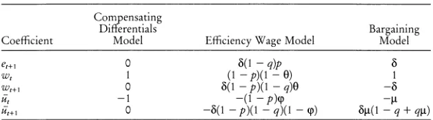
about the He's and their relationship to the underlying structural parameters are summarized in table 1.

One problem with (20) is that it includes the unobserved expectations of future variables. We deal with this in the now conventional way of invoking rational expectations and replace expectations by their actual values plus an expectational error. Doing this leads to

eit = 14o + 11e,-t+?1 + 142Wit + 143Wit+l + 144ujt + N15u "t+ + it+?1, (21)

where 8t+? is a composite expectational error term satisfying Et?t+l = 0.

Now substituting the expression (18) for effort we arrive at, after some rearrangement,

Yit = Y14o + ? 14it+i + ?pit - _{N4leit+? +} s?it - v1Thklt+l

+ 'YW2wIjt + Y13wit+l + YW4ujt + YW5UIt+1 (22)

+ Y?it+l + vit + Tjvit+i + (1 - xgl)ai + other dummies.

This is the equation that we will estimate.

Table 1

Structural Parameters of the Three Dynamic Models of Worker Effort Determination

Comipensating

Differentials Bargaining

Coefficient Model Efficiency Wage Model Model

et+ I?0 6(1 - _q)p 6

&7t 1 (1-p)(1-0) 1

Wt+ I 0 6(1 - p)(1 - q)O -6

Ut -1 -(1 - p) -g

Ut+ I 0 -6(1 - p)(1 - q)(1 - p) 6g(1 - q + qg)

NOTE.-Explanation of parameters: 8 discount factor; q = quit rate; p = probability of shirker not being caught; 0 = probability of being paid current wage for caught shirker; (p = probability of receiving

There are several points that need discussing. First, to eliminate firm- specific effects, we will estimate (22) in first differences. This means that the earliest legitimate instruments will be those of date (t - 2). Second, consider the nature of the error term in (22). If v., the errors in the pro- duction function are white noise, the error in (22) will, after first differ- encing, possibly have an MA(1) structure (depending on the correlation between cit and v1t).. If, instead, vit has an AR(1) structure, then the error in (22) will possibly have an ARMA(1, 1) structure. Given that the pro- cedure of estimating in first differences will tend to induce first-order au- tocorrelation in the equation error, we are careful to test for the presence of second-order residual autocorrelation in our equations and to check whether the first-order residual covariance is close to 0.5, which is what we would expect if the errors in (22) are white noise.

The identification of (22) also deserves some discussion. What we are estimating are the wage-effort combinations at which effective labor will be available to the firm. An attempt to pay workers a lower wage, for example, would in the compensating differentials model cause workers to quit, in the union model it would cause them to strike, and in the efficiency wage model it would cause them to shirk. So, what we are estimating is really the supply curve of labor to the firm. One worry about identification might be the following. If firms were on their labor demand curves, and if, for example, the technology had a constant elasticity of substitution, then labor productivity would be positively related to the real product wage. We need to ensure that when we estimate (22), we are not estimating this type of relationship. To identify (22) as the supply curve of labor to the firm we need to use as instruments variables that will influence labor demand (and the choice of effort) but that do not directly enter into (22). One obvious instrument is the product wage; as our theories concern the supply side, the wage variable is the consumer wage. But, as available measures of product prices are less than ideal (i.e., not at firm level), we also use profits as an instrument as they will be influenced by the product price and other factors shifting demand for the firm's product.

Finally, another issue is why we use an approach based on direct esti- mation of the production function. One might also think of estimating factor demands that will, in general, depend on worker effort and then eliminate effort in the way that we did above to derive an estimable Euler equation (Green and Weisskopf [ 1990] follow a somewhat similar approach when they estimate hours equations based on a "cost-of-job-loss" model). We do not follow this approach for two reasons. First, the real product

5 One might expect that the composite error term in (22) would be almost

certain to have an MA( 1) structure because it includes both vit and vit+ . But the expectational error sit+, is almost certainly strongly correlated with vit+l, making

wage will enter factor demands directly, and this will affect the predicted signs on our coefficients, making our tests much less clear-cut and causing more serious problems with identification. One could distinguish between product and consumer wages, but given the lack of good measures of product prices this is unlikely to be very satisfactory. And if there is some kind of bargaining by unions over the level of employment (as, e.g., in the efficient bargaining model of McDonald and Solow [1981]), the alternative utility level will also appear directly in factor demands (see Nickell and Wadhwani [in press] for a fuller discussion of this).

Second, we know that dynamics are very important in factor demands,

and if we are estimating Euler equations, it is very important that these dynamics are modeled properly (see Machin, Manning, and Meghir [1991] for one approach using essentially this data set).

For these reasons, we believe that estimating production functions di- rectly offers the best hope of a clear-cut test of the hypotheses in which we are interested, and this is the approach that we take.

IV. The Data

The data we use are an unbalanced panel of 486 U.K.-quoted companies drawn from the Datastream data bank, over the period 1976-86. The bal- ance of the panel is such that we have 253 firms with 7 years data, 52 with 8, 44 with 9, 89 with 10, and 48 with 11. This is the same data source as used by Wadhwani and Wall (in press) in their study.

Accounts data are clearly attractive in that they give us a panel aspect, although they do have some shortcomings. In particular, we are forced (like Wadhwani and Wall) to model yit as the log of real sales as we do

not have data on value added. The variables kit and lit are measured by

capital stock and total U.K. employment data, while wit is the log of the average real wage in the firm. The variable wit is defined as [(1 - urt)wt + urtbtj, where wt is the log of the industry wage and ur and b are the aggregate unemployment rate and benefit levels, respectively.

The reported models are estimated in first differences to remove fixed effects using instrumental variable methods designed for unbalanced panels, as described by Arellano and Bond (1991). Effectively, this amounts to using an optimal set of instruments to obtain efficient parameter estimates (in the absence of serial correlation). Tests of instrument validity are also presented to ensure the instrument set used is uncorrelated with the resid- uals of the equation.

V. Results

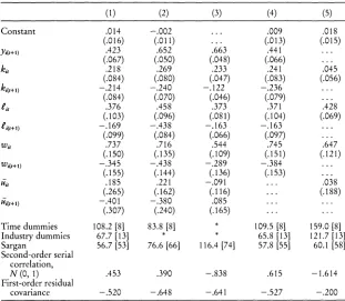
Table 2

Unrestricted Models

(1) (2) (3) (4) (5)

Constant .014 -.002 ... .009 .018

(.016) (.011) ... _{(.013) (.015)}

Ya(t+1) .423 .652 .663 .441 ...

(.067) (.050) (.048) (.066) ...

kit .218 .269 .233 .241 .045

(.084) (.080) (.047) (.083) (.056)

k,(t+,) -.214 -.240 -.122 -.236 ...

(.084) (.070) (.046) (.079) ...

-eit .376 .458 .373 .371 .428

(.103) (.096) (.081) (.104) (.069)

e,(t+I) -.169 -.438 -.163 -.163

(.099) (.084) (.066) (.097) ...

wit .737 .716 .544 .745 .647

(.150) (.135) (.109) (.151) (.121)

W,(t+1) -.345 -.438 -.289 -.384 ...

(.155) (.144) (.136) (.153) ...

ait .185 .221 -.091 ... .038

(.265) (.162) (.116) ... (.188)

ui(t+I) -.401 -.380 .085 ... ...

(.307) (.240) (.165) ... ...

Time dummies 108.2 [8] 83.8 [8] * 109.5 [8] 159.0 [8]

Industry dummies 67.7 [13] * * 65.8 [13] 121.7 [13]

Sargan 56.7 [53] 76.6 [66] 116.4 [74] 57.8 [55] 60.1 [58]

Second-order serial correlation,

N (0, 1) .453 .390 -.838 .615 -1.614

First-order residual

covariance -.520 -.648 -.641 -.527 -.200

NOTE.-Number of firms = 486. N = 2,543. The dependent variable is yit. Asymptotic standard errors

are in parentheses. All models are estimated in the first differences using Arellano and Bond's (1991) two- step instrumental variable estimator. All variables are instrumented using lags dated (t - 2) for each period on all variables (eight instruments per variable from 1979-86), (t - 3) each period on k and e, and all models include (t - 2) dated profits as outside instruments. A Sargan x2 test of the implied overidentifying

restrictions is also reported (degrees of freedom in brackets). A test for second-order serial correlation is presented: it is a N (0,1 ) statistic (see Arellano and Bond 1991). Wald tests of the significance of including

industry or time dummies are presented where they were included (degrees of freedom in brackets). * Estimates omitted from model.

both industry and time dummies, while column 4 includes both and omits the alternative utility level.

In all cases the results are very similar. First, there is no evidence of second-order residual autocorrelation in any of the equations, and the first-order residual covariance is always close to -0.5, indicating that the hypothesis that the errors in (22) are white noise is acceptable. Second, the coefficients on y, k, and

e

6 _{The estimated elasticity of output with respect to the capital stock is on the}

factor inputs suggest that the approach we have adopted is a broadly sen- sible one.

Now consider which of the three theories we have considered is more supported by the data. First, consider the compensating differentials model. This predicts that all the future variables should be insignificant. It is not hard to see that these restrictions are rejected. More formally, column 5 presents estimates of a static model. And Wald tests for the exclusion of the future terms from columns 1-4 range from x2(5) = 47.3 for column I to x2(5) = 325.9 for column 3.

Second consider the efficiency wage model. This predicts that the coef- ficients on current and future wages should both be positive while those on the current and future alternative utility level should both be negative. From the inspection of the coefficient on wit+, in all the equations it can be seen that this prediction finds little support here.

The predictions of the collective bargaining model do, however, get more support. The coefficients on current and future wages are exactly as predicted, and while the coefficients on the alternative wage are the opposite to those predicted, these coefficients are insignificant. This is not too sur- prising given that a substantial part of the alternative wage may be captured by the time dummies. Indeed, when we omit the time dummies in column 3, the signs on the alternative wage terms are consistent with the bargaining model, although they are not large enough in absolute terms. However, the x2 test of the overidentifying restrictions implied by the instrument set fails in column 3. Furthermore, it should be noted that the time dummies are always jointly significant even when the alternative utility level is in- cluded.

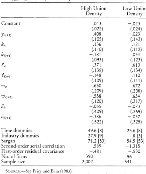
But the conclusion that the bargaining model best explains the data may be too premature. We split the sample into industries with high and low unionization using, after some experimentation, a dividing line of 50% union density in 1979. The data for industry union density are taken from Price and Bain (1983). The results are presented in table 3.

The most striking difference is that now the sign on the future wage is significantly positive in the low union density sample while it remains significantly negative in the high union density sample. This is consistent with the plausible view that the efficiency wage model is more relevant for firms in which unions are weak and that the bargaining model is more relevant for models in which unions are strong. The parameter estimates in table 3 provide some other evidence for this view. The coefficients on future output and the future wage are higher in the high union density sample, which is what our theory predicts (look at table 1). But, as before, the coefficients on the alternative utility level do not conform to either theory (although they are insignificant).

Table 3

Disaggregation by Industry Unionization

High Union Low Union

Density Density

Constant .043 -.023

(.022) (.024)

Yi(t+l) .408 -.023

(.105) (.143)

kit .136 .121

(. 1 10) (.112)

ki(t+1) -.181 .034

(.093) (.123)

fit .371 .613

(.138) (.154)

lei(t+) I-.148 .110

(.109) (.141)

wit .650 .672

(.209) (.208)

Wi(t+l) -.558 .634

(.120) (.317)

Uit -.055 -.073

(.409) (.269)

Ui(t+ 1) -.386 -.037

(.522) (.325)

Time dummies 49.6 [8] 25.6 [8]

Industry dummies 27.9 [9] .8 [3]

Sargan 71.2 [53] 54.5 [53]

Second-order serial correlation .589 -1.315

First-order residual covariance -.481 -.530

No. of firms 390 96

Sample size 2,002 541

SOURCE.-See Price and Bain (1983).

NOTE.-As for table 1. High (low) union density refers to industries with

unionization above (below) 50% in 1979.

reluctant to do because our sample split is imperfect with the result that, for example, our high (low) union density sample almost certainly contains some firms for which the efficiency wage (bargaining) model is relevant, and this would bias our estimates of the underlying structural parameters. Our conclusions are that we do have some evidence that, in firms where unions are not very powerful, the efficiency wage model does seem relevant while a bargaining model seems better for firms with powerful unions. We are cautious about our conclusions because it is conceivable that other models could explain these results. For example, a model of rent sharing, which is another form of a bargaining model, would probably imply some- thing very similar, as would a model of intertemporal substitution.7 How- ever, the fact that our results depend on the sample split we have used makes us believe that our conclusions are not entirely unjustified.

7 _{Another possibility that might be suggested to explain our results is the com-}

VI. Conclusion

This article has extended the recent literature on the empirical impli- cations of alternative models of the labor market. We have pointed out that, although these alternative models are often predicted to have the same long-run comparative statics, one can develop different predictions from these theories if one estimates empirical models derived from simple dynamic versions of the theories. The evidence that we have provided is consistent with the shirking version of the efficiency wage model for firms where unions are not very important (a minority of firms in our sample), but the bargaining model seems better for firms in highly unionized in- dustries. We are not surprised by this result. Collective bargaining is very important in the large British firms in our sample, and it is not particularly credible to believe that only the threat of shirking keeps wages high. References

Akerlof, G. A. "Labor Contracts as Partial Gift Exchange." QuarterlyJour- nal of Economics 97 (1982): 543-69.

Akerlof, G. A., and Katz, L. "Workers' Trust Funds and the Logic of Wage Profiles." Quarterly Journal of Economics 104 (1989): 525-36.

Arellano, M., and Bond, S. "Some Tests of Specification for Panel Data: Monte Carlo Evidence and an Application to Employment Equations." Review of Economic Studies 58 (1991): 277-98.

Gibbons, R., and Katz, L. "Unmeasured Ability and Inter-industry Wage Differences." Working paper. Cambridge, Mass.: National Bureau of Economic Research, October 1989.

Green, F., and Weisskopf, T. E. "The Worker Discipline Effect: A Dis- aggregative Analysis." Review of Economics and Statistics 72 (1990): 241 - 49.

Krueger, A., and Summers, L. "Efficiency Wages and the Inter-industry Wage Structure." Econometrica 56 (1988): 259-93.

McDonald, I., and Solow, R. "Wage Bargaining and Employment." Amer- ican Economic Review 71 (1981): 896-908.

Machin, S.; Manning, A.; and Meghir, C. "Dynamic Models of Employment Based on Firm Level Panel Data." Working paper. London: London School of Economics, September 1991.

Macleod, W. B., and Malcomson, J. M. "Implicit Contracts, Incentive Compatibility and Involuntary Unemployment." Econometrica 57 (1989): 447-80.

Malcomson, J. M. "Work Incentives, Hierarchy and Internal Labor Mar- kets." Journal of Political Economy 92 (1984): 486-507.

Murphy, K. M., and Topel, R. "Unemployment, Risk and Earnings." In Unemployment and the Structure of Labor Markets, edited by K. Lang and J. Leonard. London: Basil Blackwell, 1987.

Nickell, S., and Wadhwani, S. "Employment Determination in British Industry: Investigations Using Micro-data." Review of Economic Studies (in press).

Nickell, S.; Wadhwani, S.; and Wall, M. "Unions and Productivity Growth in Britain, 1974-86: Evidence from U.K. Company Accounts Data." Discussion Paper no. 353. London: London School of Economics, Centre for Labour Economics, August 1989.

Price, R., and Bain, G. S. "Union Growth in Britain: Retrospect and Pros- pect." British Journal of Industrial Relations 21 (1983): 46-68.

Shapiro, C., and Stiglitz, J. E. "Equilibrium Unemployment as a Worker Discipline Device." American Economic Review 74 (1984): 433-44. Stewart, M. "Union Wage Differentials in the Face of Changes in the

Economic and Legal Environment." Economica 58 (1991): 155-72. Wadhwani, S., and Wall, M. "A Direct Test of the Efficiency Wage Model

Using U.K. Micro-data." Oxford Economic Papers (in press).