INTERNATIONAL JOURNAL OF ADVANCE RESEARCH IN SCIENCE
AND ENGINEERING (IJARSE)
Introduction to Image processing using MATLAB
Abstract—We live in a visually enchanting world which build itself with variety of shapes, size, colours etc. This vision is very important for humans they are capable of acquiring, integrating, interpreting and processing this heavy amount of visual information around them. Without vision human life is very difficult.
Image processing is all about changing the nature of image for our convenience. Here is a paper presenting some of the essential details of image processing and some of the techniques of image processing using MATLAB. Some applications are also been discussed at the end of the paper.
The main thrust of the paper is to help the beginners of this field to understand the topic “image processing” and use it with MATLAB.
Index Terms— Image processing, Digital image processing, MATLAB, image processing using MATLAB, image enhancement technique, image smoothening.
INTRODUCTION
Humans are predominantly visual creatures; they rely heavily on their vision to make sense of the world around them. They have capability to acquire, integrate, interpret and process this heavy amount of visual information around them. It is challenging to impart such capabilities to a machine. But we have to do this difficult task in accordance to capture the images of this world. And to see these images more clearly and more suited to our vision we have to apply image processing to it.Image processing is all about manipulating the nature of input image in accordance to improve its pictorial information for human perception [1]. Image processing can be either in analogue or in digital but digital image processing is better than analogue due to its certain advantages. Thus digital image processing is more popular. In digital image processing we process digital images by the means of computer algorithms [2].
Some examples of image processing can be as follows:
(a) noisy image (b) Image after removal of noise
*Fig.1- Removing the noise from the image (noise is the common problem in data transmission)
(a) Original image (b) Blurred image *Fig.2- Removing details from the image
(a) Original image (b) After removal of motion blur Fig.3- Removing motion blur
Analog and digital images
Fig.5- Image as a function
In such images we may assume that the image brightness value may be taken as any real value ranging from 0.0(black) to 1.0(white) depending upon the image.
In Digital image values of x, y are discrete. They can take any integer value ranging from 0(black) to 255(white). It can be considered as a large array of discrete dots each of which has a brightness associated with it. These dots are called picture element or more simply pixels.
Fig.6-Pixels in grey level image
Classes of digital images
a) Binary images- in these images there can be only two values of each pixel either 0(black) or 1(white). This type of coding scheme is best suited for text, finger prints or architectural plans. These are very convenient in terms of storage.
*Fig.7- Binary image
a) Images- To understand easily the concept of images let us take grey scale images so that our analysis gets simpler. An analog image may be defined as a 2 dimensional function of the brightness of the image at any given point as shown in the figure 5. Means each pixel may be represented by 1 byte. These sorts of images are used in medical industry (x-ray) etc.
Fig.8-Grey scale image
MATLAB do not distinguish between a grey scale image and binary image. It consider binary image an special case of grey scale image.
b)RGB coding- This coding scheme produces what is known as true colour image. Here each pixel has a particular colour which is being described by the intensity of red, green and blue in it. Now each of the component has a range of 0 to 255, thus the total colour combination can be 2553=16,777,216 different colours in the image. Such an image may be considered as the stack of three matrices representing red, green and blue values for each pixel [1].
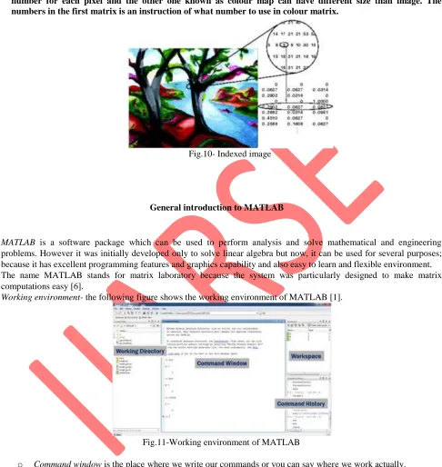
c) Indexed image- in this an image is stored as two matrices. First have the same size as the image and one number for each pixel and the other one known as colour map can have different size than image. The numbers in the first matrix is an instruction of what number to use in colour matrix.
Fig.10- Indexed image
General introduction to MATLAB
MATLAB is a software package which can be used to perform analysis and solve mathematical and engineering problems. However it was initially developed only to solve linear algebra but now, it can be used for several purposes; because it has excellent programming features and graphics capability and also easy to learn and flexible environment. The name MATLAB stands for matrix laboratory because the system was particularly designed to make matrix computations easy [6].
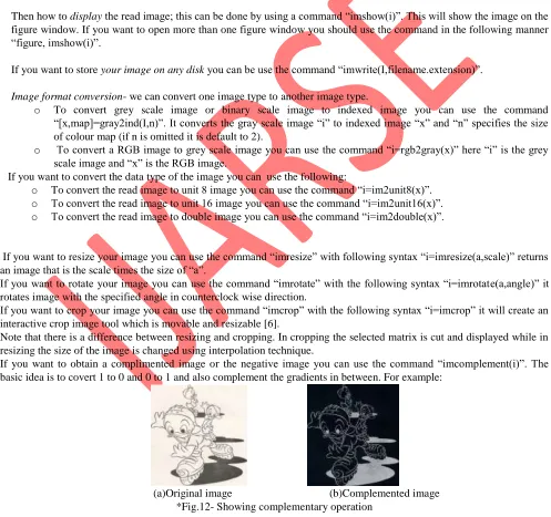
Working environment- the following figure shows the working environment of MATLAB [1].
Fig.11-Working environment of MATLAB
o Command window is the place where we write our commands or you can say where we work actually.
o Working directory is the place where all our files we have to work with are stored. And the most important thing to work in MATLAB is that the file you want to work with should be present in its working directory otherwise the file does not exist for MATLAB.
o Workspace is the place where all the variables you use in command window are created. If you store something new to the same variable it will overwrite the previous value.
o Command history is the place where all the work you have done in command window, history of its is displayed.
Image processing using MATLAB
In MATLAB digital images are represented in the form of matrix. For a grey scale image it is a two dimensional matrix and for a coloured image it is a multi dimensional matrix [1].
To apply image processing to any image first of all we should know how to give it as an input. In MATLAB images can be read using a command “imread”. Its syntax is i=imread(„file name.extension‟).But this filename.extension must be present in your working directory then only MALAB will read the pixel values of the image and stores a matrix of all the pixel values in the variable “i” which will be shown in the workspace. It is advisable that this command should be ended with semicolon. Semicolon at the end of the command will prevent the obtained matrix to be displayed on command window. If you want to find out the size of the image the command is “size(i)”. To read an indexed image command is “[x,map]=imread(„filename.extension‟)”.
Then how to display the read image; this can be done by using a command “imshow(i)”. This will show the image on the figure window. If you want to open more than one figure window you should use the command in the following manner “figure, imshow(i)”.
If you want to store your image on any disk you can be use the command “imwrite(I,filename.extension)”.
Image format conversion- we can convert one image type to another image type.
o To convert grey scale image or binary scale image to indexed image you can use the command “[x,map]=gray2ind(I,n)”. It converts the gray scale image “i” to indexed image “x” and “n” specifies the size of colour map (if n is omitted it is default to 2).
o To convert a RGB image to grey scale image you can use the command “i=rgb2gray(x)” here “i” is the grey scale image and “x” is the RGB image.
If you want to convert the data type of the image you can use the following:
o To convert the read image to unit 8 image you can use the command “i=im2unit8(x)”.
o To convert the read image to unit 16 image you can use the command “i=im2unit16(x)”.
o To convert the read image to double image you can use the command “i=im2double(x)”.
If you want to resize your image you can use the command “imresize” with following syntax “i=imresize(a,scale)” returns an image that is the scale times the size of “a”.
If you want to rotate your image you can use the command “imrotate” with the following syntax “i=imrotate(a,angle)” it rotates image with the specified angle in counterclock wise direction.
If you want to crop your image you can use the command “imcrop” with the following syntax “i=imcrop” it will create an interactive crop image tool which is movable and resizable [6].
Note that there is a difference between resizing and cropping. In cropping the selected matrix is cut and displayed while in resizing the size of the image is changed using interpolation technique.
If you want to obtain a complimented image or the negative image you can use the command “imcomplement(i)”. The basic idea is to covert 1 to 0 and 0 to 1 and also complement the gradients in between. For example:
Some techniques of image processing using MATLAB
Following are some of the techniques of image processing:
1. Image smoothening technique- generally smoothing of the image is done in order to remove the noise. It can be done by using spatial smoothening filters. Simplest type of filter is simple averaging filter; in this simply the average of all the pixels in a neighbourhood around a central value is taken. For every pixel this process is repeated and thus a smoothened image is obtained.
The other type of smoothening filter is weighted smoothening filter. This is more effective technique. In this the pixel closer to the central pixel are given more value [1]. Through following images this can be seen that greater is the size of filter more is smoothening.
(a) (b)
(c) (d)
(e) (f)
*Fig.13-(a)Original image (b)Smoothened image using averaging filter of size 3 (c) Smoothened image using averaging filter of size 5 (d) Smoothened image using averaging filter of size 9 (e) Smoothened image using averaging filter of size
For image smoothening following commands has been used (for filter of size 5): i=imread(„mickey.jpg‟);
h=ones(5,5)/25; i2=imfilter(i,h); figure,imshow(i); figure,imshow(i2);
Here there are 2 new commands “ones” and “imfilter”. Command “ones(5,5)” is used to create a matrix of 5X5 and “imfilter” is used to perform the operation of filtering.
1. Filtering-It is usually done to remove noise from the images. Noise is the common problem in transmission. If you transmit images noise can be added in the communication channel. To remove the noise let us first add noise to the original image. It can be done using the command “imnoise” in following manner:
i=imread(„mini.jpg‟); g=imnoise(i,‟salt & pepper‟); figure,imshow(i);
figure,imshow(g);
You will obtain figure 12 (a), (b). Now the noise is added to the figure, so we have to apply the filtering operation to remove it. Filtering can be done using the command “imfilter”. Let us take the following filter „h‟ and then remove the noise from image.
h=[1/9 1/9 1/9;1/9 1/9 1/9;1/9 1/9 1/9]; i2=imfilter(g,h);
figure,imshow(i2);
Now we will obtain the final image after removal of noise (figure 14(c)).
(a)Original image (b) Image after adding noise.
(c)Image after removal of noise
*Fig.14- Removing the noise from the image (noise is the common problem in data transmission)
1. Image enhancement techniques- it lies under the category of spatial filtering. Image enhancement includes highlighting the fine details, removing the blurring from the image and highlighting the edges. Sharpening is obtained by sharpening spatial filters, which is based on spatial differentiation. Differentiation is the measure of rate of change of a function [1].
useful for image enhancement than the first derivative. The laplacian operator is an example of second order derivative method [5].
By applying the laplacian to an image we get an image highlighting the edges and other discontinuities as shown below.
(a) Original image (b) Laplacian filtered image *Fig.15- showing the Laplacian operation on image
For edge detection or laplacian filtered image following commands has been used [6]: i=imread(„jack.jpg‟);
h=[0 1 0;1 -4 1;0 1 0]; i2=imfilter(I,h); figure,imshow(i); figure,imshow(i2);
But this is not the required enhanced image after laplacian filtering, we have to do more. We have to subtract the laplacian resulted image from the original image to get the enhanced image [5].
After the above command, to get the final image you can simply write the following commands:
g=i-h;
figure,imshow(g); then you will obtain the figure 14(c)
(a)Original (b)Laplacian filtered (c)Enhanced image
*Fig.16- laplacian image enhancement
*These images has been processed by me using MATLAB
some applications of image processing
Image processing can be used in almost every field of science and technology. Some of the examples are as follows: a. Biomedical applications- it is mainly used interpreting the things for diagnosis. Like CT scan, X-rays, MRI, analysis
of cell images etc [2].
Fig.16- CT scan
b. Agriculture industry- we can have views of land for checking that how much land is been used for different purposes, or to investigate the suitability of different regions of land for different crops, inspecting quality of fruits and vegetables etc [1].
c. Law enforcement- we can match the fingerprints, remove the blurredness from the speed camera images etc. d. Defence surveillance- application of image processing techniques in this field is an important area of study.
There is a continuous need of monitoring land and oceans using aerial surveillance techniques.
e. Video processing- video processing is nothing but a kind of image processing. A video is made of thousands of frame of images. Thus to process a video one need to process those thousands of frame of images. Thus video processing is also one of the major applications of image processing.
Image processing can be applied in many other fields as well according to our requirements like graphic cards, video games etc.
Conclusion
Through this paper, one can have a good introduction to image processing and MALAB as well. Some image processing techniques (e.g. Image smoothening technique and enhancement techniques) for digital image enhancement and some MATLAB commands for image processing have been studied in the paper using MATLAB. We can also conclude that greater is the size of the filter greater is the smoothening.
A lot more work is needed in this field to develop new technologies in future to reduce the complexity and increase the quality of the image.
REFERENCES
[1] http://Orane labs.com/.
[2] Tinku Acharya and Ajoy K.Ray, ”Image processing-principles and application”. Wiley interscience,2006.
[3] Bolhouse, V., “Fundamentals of Machine Vision” Robotic Industries Assn, 1997.
[4] Parker, J., R., “Algorithms for Image Processing and Computer Vision”, Wiley Computer Publishing, 1997.
[5] Gonzales and Woods, “Digital image processing”, second edition, Prentice Hall Publisher, 2002.