Collusion Resistant Traitor Tracing from Learning with Errors
Rishab Goyal
UT Austin
[email protected]
Venkata Koppula
UT Austin
[email protected]
Brent Waters
UT Austin
[email protected]
∗Abstract
In this work we provide a traitor tracing construction with ciphertexts that grow polynomially in log(n) where n is the number of users and prove it secure under the Learning with Errors (LWE) assumption. This is the first traitor tracing scheme with such parameters provably secure from a standard assumption. In addition to achieving new traitor tracing results, we believe our techniques push forward the broader area of computing on encrypted data under standard assumptions. Notably, traitor tracing is substantially different problem from other cryptography primitives that have seen recent progress in LWE solutions.
We achieve our results by first conceiving a novel approach to building traitor tracing that starts with a new form of Functional Encryption that we call Mixed FE. In a Mixed FE system the encryption algorithm is bimodal and works with either a public key or master secret key. Ciphertexts encrypted using the public key can only encrypt one type of functionality. On the other hand the secret key encryption can be used to encode many different types of programs, but is only secure as long as the attacker sees a bounded number of such ciphertexts.
We first show how to combine Mixed FE with Attribute-Based Encryption to achieve traitor tracing. Second we build Mixed FE systems for polynomial sized branching programs (which corresponds to the complexity class logspace) by relying on the polynomial hardness of the LWE assumption with super-polynomial modulus-to-noise ratio.
1
Introduction
In a (traitor) tracing [CFN94] system an authority runs a setup algorithm that takes in a security parameter
λ and the number, n, of users in the system. The setup outputs a public key pk, master secret key msk, andnsecret keys (sk1,sk2, . . . ,skn). The system has an encryption algorithm that uses the public keypkto
create a ciphertext for a messagemthat is decryptable by any of thensecret keys, but where the message will be hidden from any user who does not have access to the keys. Finally, suppose that some subsetS of users collude to create a decoding boxDwhich is capable of decrypting ciphertexts with some non-negligible probability. The tracing property of the system states that there exists an algorithmTrace, which given the master secret and oracle access toD, outputs a set of usersT where T contains at least one user from the colluding setS and no users outside ofS.
Existing approaches for achieving collusion resistant broadcast encryption can be fit in the framework of Private Linear Broadcast Encryption (PLBE) introduced by Boneh, Sahai, and Waters (BSW) [BSW06]. In a PLBE system the setup algorithm takes as input a security parameter λand the number of users n. It outputs a public keypk, master secret keymsk, andnprivate keyssk1,sk2, . . . ,sknwhere a user with indexj
is given keyskj. Any of the private keys is capable of decrypting a ciphertextctcreated usingpk. However,
there is an additional TrEncrypt algorithm that takes in the master secret key, a message and an index i. This produces a ciphertext that only users with indexj > ican decrypt. Moreover, any adversary produced
∗Supported by NSF CNS-1228599 and CNS-1414082. DARPA through the U.S. Office of Naval Research under Contract
decryption boxD that was created with private keys in the set ofS will not be able to distinguish between encryptions to indexi−1 or i, wherei /∈S. In addition, encryptions of two different messagesm0, m1 to indexnmust be indistinguishable.
The tracing system is setup by simply running the PLBE setup and distributing each PLBE key to the corresponding user. To trace the set of colluding parties given a decoding boxD, the tracing algorithm first measures (with several samples) the probability thatD correctly decrypts a ciphertext encrypted to indexi
for all i∈[0, n]. If the boxD originally decrypted with probability , then there must exists some index i
where the probability the box decrypts on indexi−1 is at least/nmore than the probability it decrypts on ciphertexts encrypted to indexi, as by PLBE securityD can not decrypt encryptions to index n with non-negligible probability. At this point the tracing algorithm marks userias a colluder.
Currently, there are three approaches to building PLBE. The most basic approach is to simply createn
public/private key pairs under a standard IND-CPA secure public key encryption system. A PLBE ciphertext is formed by encrypting the message m to each user’s public key individually and concatenating all of the sub-ciphertexts to form one long ciphertextct= (ct1,ct2, . . . ,ctn). A user with secret keyski in the system
will decrypt by running decryption oncti and ignore the rest of the ciphertext components. ToTrEncryptto
indexisimply encrypt the all 0’s string in first iciphertextsct1, . . . ,cti in place of the message. The index
hiding property follows directly from IND-CPA security of the underlying encryption scheme as without secret keyi no attacker can distinguish whethercti is an encryption of the message or all 0’s string.
The above approach works because there is a portion of the ciphertext cti dedicated to each useri in
the system which is not touched during the decryption process of other users with keysskj forj6=i. This
dedicated ciphertext space strategy makes it easy to silently kill useri’s ability to access the message in a way unnoticeable to other users, but also inherently requires a ciphertext size that grows linearly in n. In order to achieve PLBE with sublinear size ciphertexts one needs to implement some form of computing on encrypted data.
BSW [BSW06] provided the first construction that achieved PLBE with ciphertext growth that was sub-linear inn. They leveraged composite order bilinear groups to achieve ciphertexts that grew proportionally to √n. While future variants [BW06, GKSW10, Fre10] used bilinear maps to obtain additional properties, the ciphertext size for all bilinear-map based constructions remained stuck at the√nmark.
Several years later Boneh and Zhandry [BZ14] showed how to utilize indistinguishability obfuscation and apply punctured programming techniques to achieve the ideal case where ciphertexts grow polynomially in log(n) andλ. The downside of applying indistinguishability obfuscation is that all current obfuscation candi-dates are based on non-standard multilinear map group assumptions, and several such multilinear candicandi-dates have been attacked (see [CLT14, CHL+15, CGH+15, BGH+15, CLLT16, CLLT17, BWZ14, HJ16, Hal15, CFL+16,MSZ16,CJL16,ADGM16] and the references therein). (One could also achieve similar results from
using the functional encryption scheme of Garg et al. [GGH+13], but this also relies on multilinear maps.)
This leaves open the following question:
Can we build secure traitor tracing withpoly(λ,log(n))-sized ciphertexts from standard assumptions?
Our Results
In this work we resolve the above question by providing a traitor tracing construction with ciphertexts that grow polynomially in log(n) andλand prove it secure under the Learning with Errors (LWE) assump-tion. This is the first traitor tracing scheme with such parameters that is provably secure from a standard assumption. In addition to achieving new traitor tracing results, we believe our techniques push forward the broader area of computing on encrypted data under standard assumptions. Notably, traitor tracing is substantially different problem from other cryptography primitives that have seen recent progress in LWE solutions.
encode many different types of programs, but is only secure as long as the attacker sees a bounded number of such ciphertexts.
We first show how to combine Mixed FE with Attribute-Based Encryption to achieve traitor tracing. Second we show under the LWE assumption how to construct Mixed FE systems for polynomial sized branching programs (which corresponds to the complexity classlogspace).
1.1
Technical Overview
We now give a technical overview of our work. This overview is broken into four parts. In the first part we review the BSW notion of Private Linear Broadcast Encryption and its transformation into a traitor tracing system. Along the way we discover that the PLBE definitions as presented in [BSW06] donot imply traitor tracing. We then show how to repair the argument by giving the attacker an additional oracle encryption query in the PLBE definitions. Second, we present the notion of Mixed FE and show how an ABE and Mixed FE system (for the right functionalities) can be used to construct a PLBE system. The third part of our overview describes a new LWE toolkit which includes “enhanced” versions of lattice trapdoor sampling algorithms with additional security properties. Finally, we outline our main ideas for constructing the Mixed FE system and proving it secure under the LWE assumption.
Part 1: Breaking and Repairing the PLBE to Tracing Argument. First, let us review the PLBE
algorithms as defined in [BSW06]. A PLBE scheme consists of a setup, encryption, decryption and trace-encryption algorithm. The setup algorithm outputs a public key, a master secret key and n secret keys, one for each index in [n]. The encryption/decryption algorithms are self-explanatory; the trace-encryption algorithm is a special encryption algorithm that requires the master secret key, and can be used to encrypt a message to any indexi∈[0, n]. The output ciphertext can be decrypted only by secret keys for indicesj > i. BSW defined three security properties. The first security property (public to zero-index indistinguishability) requires that a standard encryption of message mis indistinguishable from a trace-encryption of mto the index 0, even when the adversary has all the n secret keys. The second security property (index hiding) states that a trace-encryption ofmto indexi−1 is indistinguishable from a trace-encryption ofmto index
i, even when the adversary has all the secret keys except the ith one. Finally, the third security property
states that trace-encryption ofm0 to index nis indistinguishable from trace-encryption of m1 to index n, even when the adversary is given allnsecret keys.
BSW argued that these three properties of PLBE are sufficient for constructing a traitor tracing (TT) scheme. In their transformation, the TT public key and n secret keys are set to be the PLBE public key and n secret keys, respectively. The TT encryption/decryption algorithms are identical to the PLBE encryption/decryption algorithms. Finally, the tracing algorithm uses the PLBE trace-encryption algorithm. Given a decoder boxD, the tracing algorithm encrypts random messages to each index, and checks ifD can decrypt it correctly. If the decoder box is-successful1 in decrypting (standard) encryptions, then it is also successful in decrypting trace-encryptions to index 0 (via the first security property). Next, note that the decoder box cannot decrypt trace-encryptions to index n (via the message indistinguishability property). Therefore, there must exist an index i∗ ∈ [n] where the success of the decoder box in decrypting trace-encryptions to indexi∗−1 is at least/nmore than its success in decrypting trace-encryptions toi∗. This indexi∗ must be one of the indices queried by the adversary (since if the adversary does not have a key for
indexi∗, then the decoder box must not be able to distinguish between trace-encryptions toi∗−1 andi∗).
For each index i, the tracing algorithm computes an estimate of the decoder box’s success probability in decrypting random trace-encryptions for indexi. For all indicesiwhere the measured success probabilities fori−1 andiare substantially different, useriis declared to be a traitor.
TT definition and the PLBE definition. The TT definition considers an attacker that produces a (stateless) decoderDwhose success on decrypting multiple trace-encryptions is measured, whereas the PLBE definition considers indistinguishability on a single ciphertext (in particular, no ciphertext queries). Diving deeper, we show a separation by adding a feature to a PLBE scheme where the feature does not impact PLBE security, but results in an insecure TT scheme.
Given any secure PLBE scheme P, consider a schemeP0 defined as follows. The setup algorithm ofP0 is similar to the setup ofP, except it also samples an additional PRF keyK as part of the master secret key (we will assume the PRF has single bit output). The (standard) encryption algorithm computes a ciphertext ct using the underlying scheme’s encryption algorithm, chooses a uniformly random bitband outputs (ct, b). The trace-encryption of message m is the ciphertext ct0 = (ct, y = PRFK(i)) where ct is the ciphertext
obtained from the trace-encryption algorithm ofP. It is easy to see that the new scheme satisfies all three PLBE security definitions, since there are no encryption queries allowed in the PLBE scheme beyond the challenge ciphertext.
However, it is possible to construct a decoding box using only secret key for indexnsuch that the trace algorithm falsely accuses some user i < n. The decoderD, on input of a ciphertext ct0 = (ct, y), tests if
y = 1. If so, it decrypts the ciphertext using key skn; otherwise it outputs a random message. Using PRF
security, we can argue that there exists an index i < nsuch that PRFK(i−1) = 1 and PRFK(i) = 0 with
high probability. In this case the probability thatD decrypts ciphertexts for indexi−1 will be measurably different than the case it decrypts ciphertext for indexi. Thus useriwill be flagged as a colluder.
We repair the BSW transformation from PLBE to TT by considering a modified set of PLBE security definitions and prove that these do imply TT. We do so in two steps. First, we consider a decoder-based
version of the BSW PLBE definitions. For concreteness, let us consider the index hiding definition. The decoder-based version of index hiding version states that no adversary, given all secret keys except the ith
one, can produce a decoder boxD and a messagemsuch thatD can distinguish between trace-encryptions of mto index i−1 and trace-encryptions of m to indexi. Decoder-based versions of the other properties are defined similarly.
Now that we have decoder-based PLBE definitions that align with the decoder in the TT definitions, it is fairly straightforward to prove that the BSW transformation implies TT. The downside of introducing decoder-based PLBE definitions is that they are more difficult to work with as a target for a construction. We address this issue by circling back to the original (BSW) PLBE definitions, and augmenting them by allowing an attacker to make an apriori bounded number of queries to an encryption oracle. We show that 1-query PLBE implies decoder-based PLBE. This gives us an easier target (that is, 1-query PLBE).
Before describing the transformation from 1-query PLBE to decoder-based PLBE, we would like to point out that if the BSW definitions were augmented to allow an unbounded number of ciphertext queries, then decoder-based security follows immediately. For instance, let us consider the index hiding game. The reduction algorithm (that reduces unbounded-query PLBE to decoder-based PLBE) receives a decoder box
Dfrom the attacker. Given the unbounded queries, the reduction algorithm can measure (within reasonable accuracy) the success probabilities of D for indices i−1 and i, and therefore, whether it can use D to distinguish between an encryption to index i−1 and i. However, with only 1 encryption query no such precise measurement is possible. Therefore, showing an attacker on decoder-based PLBE security implies and attacker on 1-query PLBE is a bit tricky. The reduction algorithm, after receiving the decoder box and message m from the adversary, chooses a random index i∗ ∈ {i−1, i}, and queries the challenger for encryption of m for index i∗. It receives a ciphertext ct. Next, it queries the challenger with challenge message m, and receives a challenge ciphertext ct∗. The reduction algorithm checks if D(ct) =D(ct∗); if so, it guesses that mwas encrypted for indexi∗. We would like to point out that choosing query index i∗
uniformly at random from{i−1, i}(as opposed to just fixing one of the two) is important for our analysis. The complete details of our analysis can be found in Section4.1.
[BW06]), since the public key allows the reduction algorithm to generate ciphertexts.
Part 2: Constructing PLBE from Mixed FE. The hardness of constructing a PLBE scheme stems
from the fact that it needs to satisfy the following three properties at the same time. First, a PLBE scheme needs to provide an Attribute-Based Encryption (ABE) like functionality where each secret key is associated with an “index”, and each ciphertext is associated with anindex comparison predicate. Second, the scheme must provide a Broadcast Encryption (BE) like compactness guarantee which is that the size of ciphertexts must be short. Third and most importantly, it must provide a Predicate Encryption (PE) like security, that is the ciphertexts must not reveal any more information about the associated index comparison predicate other than what can be learnt by running decryption.
In this work, instead of directly building a PLBE scheme, we further reduce the task to constructing a new form of FE scheme called Mixed FE. We show how Mixed FE can be combined with ABE for circuits to obtain PLBE. At a very high level, our approach is to decouple the functionality (delivering the message to users) and security requirements of a PLBE scheme, and deal with them separately.
We begin by informally introducing the notion of Mixed FE. A Mixed FE scheme consists of a setup, normal (or public key) encryption, secret key encryption , key generation, and decryption algorithm. The setup algorithm takes as input the security parameterλand description of the function classF, and outputs the public parameters pp and the master secret key msk. The normal encryption algorithm only takes as input the public parameterspp, and outputs a (normal) ciphertextct. The secret key encryption algorithm takes as input the master secret key mskand a function f ∈ F, and outputs a (secret key) ciphertext ct. The key generation algorithm takes as input the master secret key msk and a message m, and outputs a key skm. The decryption algorithm takes as input a ciphertext ct and a secret key skm, and outputs a
single bit. Now for correctness we require that decrypting a secret key encryption of any functionf using a secret key skm outputs the evaluation of function f on message m, i.e. f(m). Whereas the decryption
algorithm (almost) always outputs 1 when given a normal ciphertext as input, irrespective of the secret key used. Thus, one could visualize the normal encryption algorithm as always encrypting a “canonical”
always-accepting function.
Intuitively, security states that no attacker should be able to distinguish between two ciphertexts that decrypt to same values under all the secret keys in attacker’s possession. Now since there are two separate encryption algorithms, we have two different security properties. The first property says that secret key encryptions of two functionsf0 andf1 should be indistinguishable if for every key in attacker’s possession, the output off0, f1is identical. We call this function indistinguishability property. The second property says that it should be hard to distinguish between a normal (public key) encryption and secret key encryption of a functionf, wheref(m) must be equal to 1 for all keys skm in attacker’s possession. We call this accept
indistinguishability property.
We show that we can construct a PLBE scheme from a (key-policy) ABE scheme and a Mixed FE scheme. The idea is to encrypt a message using the ABE system with attribute being set to be a Mixed FE ciphertext. And, each user’s secret key will be an ABE private key for the policy circuit being the Mixed FE decryption circuit with a Mixed FE secret key corresponding to user’s index hardwired. The high level intuition is that when the attribute is a normal FE ciphertext then all Mixed FE keys decrypt it to 1, thus any user with an appropriate ABE key could perform the decryption. Whereas if the attribute is set to be a secret key ciphertext, then we can control the users who can decrypt it.
Formally, the scheme works as follows. During setup, the algorithm samples both ABE and Mixed FE key pairs (abe.pp,abe.msk), (mixed.pp,mixed.msk). To compute theithuser’s private key, it samples a Mixed FE secret keymixed.ski for inputi, and also computes an ABE keyabe.ski for predicateMixed.Dec(mixed.ski,·),
i.e. Mixed FE decryption circuit with key mixed.ski hardwired. And the ABE key abe.ski is set to be
the ith user’s private key. Now to encrypt a message m, the algorithm simply runs the ABE encryption
Correctness can be observed directly. For standard PLBE ciphertext, ctattr is a normal FE ciphertext which decrypts to 1, thus the predicate Mixed.Dec(mixed.ski,·) is satisfied for all i. Therefore, by ABE
correctness, the ABE decryption algorithm will output the messagem. For PLBE indexiciphertext, ctattr is a Mixed FE secret key encryption of function ‘> i’ which decrypts to 1 for all keysmixed.skj withj > i,
thus the predicate is satisfied for all users with indices larger thani. Therefore, by ABE correctness, ABE decryption algorithm will output the message m whenever j > i. For proving security, we rely on the fact that Mixed FE ciphertexts are indistinguishable to any adversary that does not have distinguishing secret keys. For instance, suppose there exists an adversary that can distinguish between PLBE normal encryptions and index 0 encryptions, then such an adversary can also be used to distinguish between Mixed FE normal ciphertexts and secret key ciphertexts encrypting function ‘> 0’ (note that this is an always-accepting function). Thus, such an attack can be used to break accept indistinguishability property of Mixed FE scheme. Similarly, we can argue index hiding and message hiding security of the construction by reducing to Mixed FE and ABE (selective) security, respectively. Now if the Mixed FE scheme is 1-query secure, then so will be the PLBE scheme.
Now the size of ciphertexts has onlypoly-log dependence on the number of usersnas required. Because each user can be uniquely identified using a bit string of length logn, so the length of attribute (Mixed FE ciphertext) will be polynomial in logn, and thus the PLBE ciphertext which is in turn an ABE ciphertext will have length polynomial in lognas well. Also, note that to use the above transformation it is sufficient to construct a Mixed FE scheme that supports comparison operation on lognbit strings. In this work, we show how to construct a Mixed FE scheme for any class of polynomial sized branching program from the Learning with Errors assumption.2 Our construction relies only on the polynomial hardness of LWE, although we
require super-polynomial modulus-to-noise ratio. Since we already have circuit ABE schemes from the LWE assumption [GVW13,BGG+14], combining that with our Mixed FE construction we get collusion resistant
traitor tracing from the LWE assumption as well.
Looking back, it is easy to observe that Mixed FE for branching programs that supports comparison functionality is sufficient for our application. However, as a design choice, here we instead chose to construct Mixed FE for general polynomial length branching programs as it is possible that this generalization leads to more applications in the future. Moreover, focusing on logarithmic length branching programs supporting comparisons, instead of general branching programs, did not lead to any significant simplification in the Mixed FE construction or its proof.
Part 3: An Enhanced LWE Toolkit. Before describing our LWE-based construction for Mixed FE, we
define new “enhanced” properties for lattice trapdoors that will be useful in our work and we believe it will find more applications in the future. In many LWE-based works, in addition to the LWE assumption itself, a critical tool has been the notion of lattice trapdoors [Ajt99,GPV08]. Lattice trapdoor samplers consist of a pair of algorithmsTrapGenandSamplePre. The trapdoor generation algorithmTrapGenoutputs a matrix
A(that defines the lattice), and a trapdoorTA. The preimage sampling algorithmSamplePretakes as input a matrixZ, a trapdoor for matrix A, a Gaussian parameterσ and outputs a matrix Usuch thatU maps
AtoZ(that is,A·U=Z).3
These algorithms satisfy the following properties. The matrixAoutput by the trapdoor generation algo-rithm ‘looks like’ a uniformly random matrix; we call thiswell-sampledness of matrix property. Secondly, the matrix output bySamplePreis indistinguishable from a matrix drawn from a discrete Gaussian distribution with parameterσover the set of all matricesVsuch thatA·V=Z. In particular, ifZis chosen uniformly at random, then the output ofSamplePre‘looks like’ a matrixUdrawn from a discrete Gaussian distribution with parameterσ; we call this thewell-sampledness of preimage. Lattice trapdoors with these properties have found a remarkable number of applications in building LWE-based cryptography.
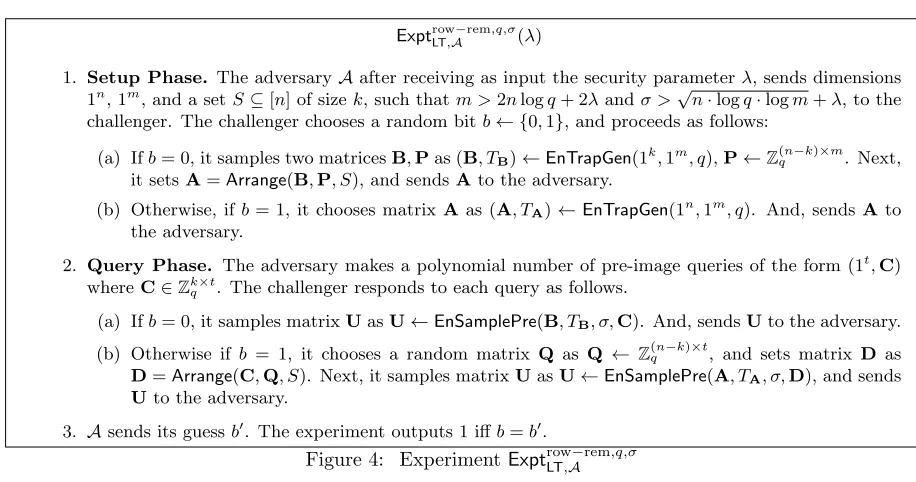
In this work, we introduce two new enhanced properties for lattice trapdoors. The first property is the
row removal property, which can be intuitively described as follows. Consider a setting where an adversary 2Note that this also gives us an alternate construction for selectively-secure private-key FE with bounded collusions [SS10,
GVW12].
specifies some ‘target vectors’, and the challenger must output a matrixAand a matrixUsuch thatUmaps some of the rows of A to the target vectors, and maps the remaining rows to uniformly random vectors. Then, these rows targetting uniformly random vectors can be removed from the trapdoor sampling. In particular, the challenger can sample a shorter matrix Bwith trapdoor, extend B with uniformly random vectors to getA, and setU to be a matrix that mapsBto the target vectors. These two scenarios will be indistinguishable for the PPT adversary.
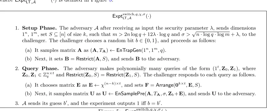
The second property is called thetarget switching property. In this setting, consider an adversary that specifies two matrices Z0,Z1 and a set of ‘target’ indices such that the rows of Z0 and Z1 agree on these target indices. The challenger is supposed to sample a matrix A with a trapdoor, compute a matrix U
that maps A to Z04 and output U together with the rows of A corresponding to the target indices and
only those rows. Then, the challenger can switch theUto map AtoZ1, and the target switching property requires that this change is indistinguishable to the adversary (note that this would not be possible if the adversary receives any of the non-target rows ofA). Moreover, the adversary is allowed to adaptively query for different target vectors/indices in both these games.
Now that we have these enhanced properties, let us discuss how to construct lattice trapdoors with these enhanced properties (using standard lattice trapdoors). Our construction is similar to theSampleLeft/SampleRight algorithms of [ABB10, CHKP10]. The enhanced trapdoor generation algorithm uses the standard trapdoor sampling algorithm to sample two matricesA1,A2together with the respective trapdoorsTA1, TA2. It
out-putsA= [A1|A2] as the matrix, andTA= (TA1, TA2) as the trapdoor. To sample a matrixUthat mapsA
toZ, the preimage sampling algorithm first chooses a uniformly random matrixW(of same dimensions as
Z). It then usesTA1 to compute a matrixU1 that mapsA1 toW, and uses TA2 to compute a matrixU2
that mapsA2toZ−W. The final preimage matrix is set to be
U1
U2
. We use the matrix well-sampledness and preimage well-sampledness of the standard lattice trapdoors to prove these enhanced properties; the detailed proof can be found in Section7.2.
Part 4: Constructing Mixed FE from LWE. Here we outline our Mixed FE construction for
polyno-mial sized (leveled) branching program from the Learning with Errors assumption. The main ingredient of our construction is the “enhanced” lattice trapdoor sampling procedure LTen = (EnTrapGen,EnSamplePre) discussed above.
First, let us recall the notion of leveled branching programs. A leveled branching program of length`and widthwcan be represented usingwstates per level, 2`state transition functionsπj,bfor each levelj ≤`, an
input-selector functioninp(·) which determines the input read at each level, and an accepting and rejecting state. The program execution starts at state st = 1 of level 1. Suppose the branching program reads the first input bit (sayb) at level 1 (i.e.,inp(1) = 1). Then, the state of the program changes fromsttoπ1,b(st).
Such a process is carried out (iteratively) until the program’s final state at level` is computed. Depending upon the final state, the program either accepts or rejects.
For ease of exposition we will start with a simpler goal of constructing a 0-query secure Mixed FE scheme for class of width-w read-once branching programs where each input bit is read once and in an ascending order. Below we first outline a construction for such a 0-query system as it contains most of the central ideas, but is easier to digest. Later we discuss the modifications with which we can improve it to be a secure 1-query scheme (and more generally, q-query secure for any polynomial q) as well as expand the function class to arbitrary polynomial sized branching programs.
Moving on to our 0-query Mixed FE construction, the master secret key consists of two sets of matrices and some trapdoor information. The first set, labeled as ‘randomization’ matrices, consists of 4` matrices {Bi,b,Ci,b}i,b for i ∈ [`], b ∈ {0,1}. And, the second set, labeled as ‘program’ matrices, consists of w`
matrices{Pi,v}i,v fori∈[`], v∈[w]. Here theCi,b matrices are sampled uniformly at random from Zn×mq , whereas the remaining (randomization and program matrices) are sampled jointly with common trapdoors 4Strictly speaking, we requireUto map the target vectors ofAto the target vectors ofZ0, but the remaining vectors ofA
(per level). Basically, for each leveli∈[`], we sample a (w+ 2)n×mmatrixMi as (Mi, Ti)←EnTrapGen(1(w+2)n,1m, q).
Now eachMi matrix is parsed as fourn×mmatrices stacked on top of each other, where first two matrices
are the randomization matrices and the remaining wmatrices are the program matrices forithlevel. That
is, for eachi,
Bi,0
Bi,1
Pi,1 .. .
Pi,w
=Mi.
All ` trapdoors T1, . . . , T` are stored as the trapdoor information in the master secret key. The public
parameters, on the other hand, only include the matrix dimensions, LWE modulus and noise parameters, but none of these matrices or trapdoor information.
At a high level, the encryption and key generation algorithms will adhere to the following structure. To (secret key) encrypt a branching program, the trapdoors will be used to sample 2` low norm matrices {Ui,b}i,b (two per level) such that each matrix Ui,b encodes the corresponding state transition function by mapping/targetting leveli‘program’ matrices to leveli+ 1 ‘program’ matrices as per the transition function
πi,b. Now the secret key for an input xwill consist of `+ 1 key vectors {ti}i. The first key component t1 will contain the program matrix P1,1 (which represents the starting state) plus some randomization component generated using the level 1 randomization matrixB1,b. The remaining ` key vectors will have
two components — the first component will cancel the previous randomization component, and the second component will add new randomization terms.5 The idea is that if decryption is performed honestly, then
all the randomization terms will get cancelled and the final output will reflect the output of the branching program.
So this way the program matrices will be tied in such a manner that they encode the state transition information and they can be used to perform the branching program execution. And the randomization matrices are added to make sure that — (1) the computation is hidden at each step, and (2) if ciphertext matrices and key vectors are combined in any inadmissible way, then the randomization components do not get cancelled. Let us now look at how to execute the above ideas.
Key Generation. The key generation algorithm takes as input a stringxand generates key vectors{ti}i as follows. It chooses`uniform secret vectorssi∈Znq fori∈[`] and`+ 1 noise vectorsei∈Zmq fori∈[`+ 1].
It also chooses ashort secret vectores∈Znq, and sets key vectors as:
∀i∈[`+ 1], ti=
s1·B1,x1+es·P1,1+e1 ifi= 1 −si−1·Ci−1,xi−1+si·Bi,xi+ei if 1< i≤`
−s`·C`,x`+e`+1 ifi=`+ 1
In words, the randomization component (likewise, cancellation component) added in the ith key vector
((i+ 1)th key vector) is an LWE sample where the public matrix used depends on the ith bit of input x.
Looking ahead, choosing the ‘randomization’ matrices depending on the stringx would assert that the ci-phertext matrices can not be arbitrarily combined to learn meaningful terms.
Normal Encryption. The normal (public key) encryption algorithm simply samples 2` random short matrices{Ui,b}i,b asUi,b←χm×m, whereχ is the noise distribution chosen during setup.
Secret Key Encryption. Moving on to the secret key encryption algorithm, on input the master secret key and a branching programBP={πi,b}i,b,acc,rej
, it samples low norm matrices{Ui,b} as follows. It
first chooses two ‘program’ matrices for last level`+ 1 asP`+1,rej=0n×mand P`+1,acc ←Zn×mq . That is,
for accepting state, it chooses a random program matrix, and for rejecting state it sets the matrix to be all zeros. Next, using theithtrapdoorTi(included in the master secret key) it runs theEnSamplePrealgorithm
to sample the ciphertext (transition) matricesUi,0,Ui,1 such that they map/target matrixMi as follows: Bi,0 Bi,1 Pi,1 .. . Pi,w Ui,0 −−−→ Ci,0 $
Pi+1,πi,0(1)
.. .
Pi+1,πi,0(w)
, Bi,0 Bi,1 Pi,1 .. . Pi,w Ui,1 −−−→ $ Ci,1
Pi+1,πi,1(1)
.. .
Pi+1,πi,1(w)
.
Here we use ‘$’ to denote a uniformly randomn×mmatrix of appropriate dimension. In words, the structure we enforce here is that the matrix Ui,b targets the Bi,b randomization matrix to itsCi,b counterpart, and the Bi,1−b randomization matrix to a random matrix. Additionally, Ui,b encodes the information about
transition function πi,b by targetting the level i program matrices to their level i+ 1 counterparts as per
πi,b. Thus, from the perspective of both correctness and security, this guarantees that a key vector ti for
some inputxmust be combined with ciphertext componentUi,xi as otherwise randomization matrix would be mapped to a random matrix, thereby destroying the underlying structure.
Decryption. First, let us focus on decrypting a secret key encryption of branching program BPusing a secret key {ti}i corresponding to an input x. Intuitively, one could visualize the matrices {Ui,0,Ui,1}i in
the ciphertext as “encodings” of the branching program state transition functions πi,0, πi,1 (respectively). Therefore, decrypting the ciphertext using secret key for some input x will be analogous to evaluating the branching programsBP on input x directly. Recall that we assumed (for ease of exposition) that the branching programs are read-once and input bits are read sequentially in ascending order. Thus, the first input bitx1 is read at level 1. Then evaluation ofBPat level 1 would map the state st1 = 1 at level 1 to statest2=π1,x1(1) at level 2. Analogously, the decryptor can compute
t1·U1,x1+t2 ≈ (s1·B1,x1+es·P1,1)·U1,x1+t2.
≈ s1·C1,x1+se·P2,st2+t2.
≈
s1·C1,x1+es·P2,st2+
−s1·C1,x1+s2·B2,x2
.
≈ s2·B2,x2+es·P2,st2.
In general, if the program state at level i during execution is sti, then the decryptor will accumulate the
term of the form si·Bi,xi +es·Pi,sti by successively summing and multiplying secret key and ciphertext
components as
(· · ·((t1·U1,x1+t2)·U2,x2+t3)· · ·+ti)
This can be verified as follows. We know that the bit read at level iisxi, thus the new state at leveli+ 1
will besti+1=πi,xi(sti). Now the accumulated sum-product during decryption will be
(si·Bi,xi+es·Pi,sti)·Ui,xi+ti+1 ≈ si·Ci,xi+es·Pi+1,sti+1+
−si·Ci,xi+si+1·Bi+1,xi+1
.
≈ si+1·Bi+1,xi+1+es·Pi+1,sti+1.
Therefore, the invariant is maintained. Continuing this way, the decryptor can iteratively compute the sum-product combining all key and ciphertext components. Note that (by definition) adding in the (`+ 1)thkey
componentt`does not introduce a term likes`+1·B`+1,x`+1 to the sum-product, thus the accumulated term
at the top will be≈es·P`+1,st`+1, wherest`+1is eitheraccorrejdepending onBP(x). Finally, the decryptor
matrix for last level corresponding to rejecting state is set to be all zeros, i.e. P`+1,rej=0n×m. Therefore, ifBP(x) = 0, then the norm of the final sum-product term will be small which the decryptor can test and output 0. Otherwise, with high probability the final sum-product term will be large and it outputs 1.
By the above analysis, correctness follows in the case where ciphertext is a secret key encryption. The correctness of decryption when the ciphertext is a normal (public key) ciphertext follows from the fact that the ciphertext matrices{Ui,0,Ui,1}i are independently sampled random short matrices.
0-Query Security. To prove 0-query security of our construction, we need to argue that it satisfies both function indistinguishability as well as accept indistinguishability properties. We start by proving function indistinguishability security. Recall that in 0-query function indistinguishability security game, an adversary submits two branching programsBP(0),BP(1) and is allowed to make a polynomial number of key queries such that for each queried inputx,BP(0)(x) =BP(1)(x) (i.e., every secret key given out has same output on both the challenge programs). The adversary receives secret key encryption of eitherBP(0)orBP(1), and its goal is to distinguish between them.
Although the full security proof is technically involved, the main ideas behind our proof are very intuitive. Before diving into the proof structure, we point out that the construction described above has to be slightly modified for proving security. Below we describe our proof ideas as well as discuss the modifications required along the way.
At a high level, our idea is to “hardwire” the output of the challenge branching programs in every secret key given to the adversary. Note that the security definition states that both challenge programs must evaluate to the same value on all queried inputs, thus we only need to hardwire a single value in each key. For ease of exposition, assume that the adversary makes exactly one secret key query. (In the general case of polynomially many key queries, the proof proceeds by hardwiring the level 1 components in all secret keys, followed by level 2 hardwiring and so on.) Let {Ui,b}i,b be the challenge ciphertext and{ti}i be the secret key computed by the challenger. Our hardwiring strategy works as follows. We start by re-writing the second secret key vectort2 in terms oft1 as follows:
t2=−s1·C1,x1+s2·B2,x2+e2
=−s1·B1,x1·U1,x1+s2·B2,x2+e2
=−s1·B1,x1·U1,x1−es·P2,st2+es·P2,st2+s2·B2,x2+e2
=−(s1·B1,x1+es·P1,1)·U1,x1+es·P2,st2+s2·B2,x2+e2
=−(t1−e1)·U1,x1+es·P2,st2+s2·B2,x2+e2
Here st2 is the state of the challenge branching program encrypted (after one step is executed). Now in the above term, we can smudge the term e1·U1,x1 by appropriately choosing the noise distributions, i.e.
e2>>e1·U1,x1.
6 (Note that since we require smudging here, thus the LWE modulus qneeds to be
super-polynomial in the lattice dimension.) Thus, the second key component can be indistinguishably computed as follows without requiring any explicit knowledge of theC1,x1 matrix.
t1=s1·B1,x1+es·P1,1+e1.
t2=
−(t1−e1)·U1,x1+es·P2,st2
+s2·B2,x2+e2
Smudging
−−−−−−−−−→ t2=
−t1·U1,x1+es·P2,st2
+s2·B2,x2+e2 .
Next, we use the row removal property of our enhanced trapdoor sampling algorithms to remove the
B1,0,B1,1 rows from the first matrix M1 and instead sample these randomly. To understand why this can be done recall that in the actual construction the encryptor needs the ability to create a ciphertext for any branching program that could be chosen even after all the keys have been distributed. That is, the encryptor must be able to sample matrices U1,0,U1,1 such that they map level 1 program matrices {P1,v}v to level 2 program matrices{P2,v}v as per some transition functions{π1,b}b as well as ensure that
B1,b·U1,b = C1,b. Now since the keys contain the matricesC1,0,C1,1 and they could be given out even before matrices U1,0,U1,1 are sampled, thus matrices B1,0,B1,1 must be sampled together with {P1,v}v
such that they share a common trapdoor.
However, at this stage in the proof the challenge branching program is (selectively) fixed ahead of any secret key queries. Therefore, in this context we can sample matricesU1,0,U1,1to only map level 1 program matrices to their level 2 counterparts, and simply set the matricesC1,b as C1,b=B1,b·U1,band use these
to compute the secret keys. We would like to point out that in order to perform this row removal securely, it is important thatB1,b·U1,1−b= $, that is matricesU1,0,U1,1 map both matrices B1,0,B1,1 to random and uncorrelated matrices.
Now once we have removed the B1,0,B1,1 rows from the first matrix, we use the LWE assumption to switch the first key componentt1 to a random vector. Note that at this point since matricesB1,0,B1,1 are sampled uniformly (i.e., are no longer sampled with trapdoor information) and secret vectors1 is not used in computing the second key componentt2, thus we can apply LWE to switcht1to random, where the LWE secret iss1 and LWE public matrix will be B1,x1.
7 Concretely, using LWE we can perform the following
switch which essentially erases the information about the level 1 program matrixP1,1 from the secret keys, thereby rendering the program evaluation to start from level 2 and statest2instead.
t1=s1·B1,x1+es·P1,1+e1
LWE
−−−−−−→ t1= $.
t2=−t1·U1,x1+es·P2,st2+s2·B2,x2+e2.
Now iteratively performing thishardwiring strategy (`times) we end up switching all but last key com-ponents to be random vectors. Also, the last key component will contain the final program matrix which is either a random matrix or a zero matrix, depending on the program output. Thus, the key vectors contain no information about the ‘program’ matrices chosen during setup. At this point, the challenge matrices{Ui,b}i,b
still contain the information about the branching program encrypted in the form of mapping between leveli
andi+ 1 ‘program’ matrices, i.e. the state transition functions{πi,b}i,b. Finally, to argue indistinguishability
here (i.e., between the challenge matrices) we use the target switching property of our enhanced trapdoors. We apply a bottom-up approach to execute this change. First, note that the level 1 program matrices do not explicitly appear anywhere, except that they are used to sample the level 1 ciphertext matricesU1,0,U1,1. Thus, we can use the target switching property to switch the targets of matrices U1,0,U1,1. Observe that this now removes the information about level 2 program matrices as well as the level 1 transition functions of challenge branching programs. Next, by the same principle, we can perform the same target switching step forU2,0,U2,1and continue so on. If we keep on performing thetarget switching step this way until the top, then the challenge ciphertext will contain no information about the challenge programs (i.e., their state transition functions) thereby completing our claim of function indistinguishability.8 This completes the first
proof.
The proof of 0-query accept indistinguishability security of our construction is similar, but more technical due to the fact that we need to argue that the challenge ciphertext is indistinguishable from random short matrices.
However, for our PLBE construction, the Mixed FE scheme must handle one ciphertext query as well, and it is not clear how to prove the above construction to be 1-query secure directly. The bottleneck is the fact that in the above proof strategy wehardwireall secret key components to match the output of challenge program. Now if the adversary is allowed to make a secret key encryption query, then it is not clear that how would the challenger still program the secret key vectors. To get around this problem, we expand our system such that it consists ofλpairs of 0-query sub-systems. Very briefly, during encryption, the algorithm now also samples aλ-bit stringtagrandomly and depending on each bit oftag, it chooses one sub-system in each
7In the general case of multiple key queries the LWE public matrices will be bothB
1,0,B1,1 and LWE secret will consist of all the secret key vectorssithat are chosen independently andper key.
pair and runs the 0-query encryption for that sub-system. Now during key generation, it (linearly) secret shares the starting program across theseλpairs of sub-systems such that same secret share is used for both sub-systems in each pair. Then, it runs the 0-query key generation algorithm for all these 2λsub-systems with their corresponding secret shares as the starting program matrices. For decryption, the sub-systems chosen during encryption are combined with their counterparts in the secret keys and 0-query decryption is performed in these sub-systems along with a (linear) reconstruction on top of the output. More details are provided in the main body.9
This completes the technical overview of our construction.
Relation to recent LWE-based schemes. There have been several recent works that have advanced the state of the art in computing branching programs on encrypted data with the goal of reducing security to LWE or LWE-like assumptions [GGH15,BVWW16, BV15,GKW17b,CC17,GKW17a, WZ17]. While our construction above benefits from that lineage we wish to briefly call out a few important distinctions.
First from a purely mechanical perspective, the construction of our Mixed FE scheme is structurally very different from the constructions of the aforementioned primitives. Very briefly, in all previous constructions the evaluator multiplies a set of matrices, and sums them up to get the final output. Whereas in our construction, we do not use this ‘one-shot’ approach for evaluation. Instead, we multiply a component from the ciphertext with a secret key component, then add in another secret key component, multiply this sum with another ciphertext component and so on. Thus, our mechanism of combining the secret key and ciphertext components is much different that what was used in prior works.10
Second we structure our proof of security to hardwire the outputs for keys one level at a time until we hit the final output level in which we have the final outputs hardwired, but lost information about the program that got us there. In this sense at a high level this leveled programming proof structure much more closely resembles that of garbled circuit proofs. Thus, we need to develop new lower LWE specific techniques to match these goals. In contrast works such as [BVWW16,GKW17b,GKW17a, WZ17] have a different aim of loosing all meaningful information when a secret is not known.
1.2
Some Future Directions
Our construction of Mixed FE relied on the LWE assumption and leveraged certain algebraic properties in that setting. An intriguing question is whether there are other avenues for achieving Mixed FE. A natural path is to build Mixed FE with a garbled circuits [Yao86] backbone. If one starts with the bounded key FE scheme of Gorbunov, Vaikuntanathan and Wee (GVW) [GVW12] and flips [AGVW13,BS15,KMUW17] the semantics of message and function one can get a secret key FE scheme that is secure for an unbounded number of private keys and bounded number of ciphertexts. To make it a Mixed FE system we would somehow connect a public key mode of encryption to the scheme. One possible path is to use a “blinded” [BLSV17] form of garbled circuits as the underlying 1-bounded scheme in the GVW transformation. (Building on [DG17a,
DG17b] blinded garbled circuits were recently used to give anonymous IBE from new assumptions). It seems possible that this approach could lead to a scheme with the accept indistinguishability property if no encryption oracle queries are allowed. However, there appears to be technical difficulties in making a public key generated ciphertext indistinguishable from a master secret key generated ciphertext when the attacker gets oracle queries. That being said, we believe that a garbled circuit approach remains a plausible future direction.
We remark that even if a garbled circuit approach becomes possible, the requirement for an ABE scheme supporting circuits will still indirectly require the LWE assumption given the state of the art. In addition, 9We would like to point out that the above idea could also be used to improve the Mixed FE construction to beq-query secure for any polynomialq. The idea will be to sample tag stringstagfrom a larger alphabet instead of{0,1}. However, we only focus on 1-query security as it is sufficient for our result.
we expect that our LWE toolkit and underlying construction ideas will have future value in any case. A second interesting direction is whether there are other applications that can leverage an FE system that has a bimodal encryption where the public key and master secret key support different spaces of messages or functions. In our Mixed FE system the public key only supported the always accept function, but there could conceivably be other variants of interest.
Finally, a natural open question is to construct traitor tracing schemes with public traceability from LWE. Currently, it is unclear if achieving public tracing is an easier task than building general public key functional encryption.
1.3
Additional Related Work
Connections to differential privacy. Dwork et al. [DNR+09] showed that existence of collusion resistant traitor tracing schemes implies hardness results for efficient differentially private [DMNS06] data sanitization. In particular, they show that if there exists a traitor tracing scheme with ciphertexts of size s(λ, n), then there exists a database of sizenand a query classQof size 2s(λ,n)such that it is hard to sanitize the database
D for query class Q in a differentially private manner. Combining our LWE based construction with the result of Dwork et al. , we get an LWE-based hardness result for differentially private sanitization with query space of size 2poly(λ,logn). We note that Goyal et al. [GKRW17] and Kowalczyk et al. [KMUW17] recently achieved similar differential privacy impossibility results from the the security of bilinear map assumptions and one way functions respectively.
Weaker notions of traitor tracing. Since the notion of traitor tracing was first proposed [CFN94],
several relaxed variants have been studied in order to achieve short ciphertexts. The first natural relaxation is the bounded collusion setting, where we have an apriori boundkthat is fixed during setup, and security is guaranteed only if the adversary gets at most k secret keys. Collusion bounded systems can either be constructed via combinatorial tools [CFN94,SW98, CFNP00, SSW01,PST06, BP08], or can be algebraic and constructed under different cryptographic assumptions such as DDH [KD98, BF99, KY02a, KY02b], bilinear DDH [CPP05,ADM+07,FNP07] and LWE [LPSS14]. Recently, Agrawal et al. [ABP+17] showed a
transformation from inner product FE to collusion-bounded TT, resulting in algebraic constructions based on various assumptions such as DCR, DDH and LWE. In all the above works, the size of the ciphertext grows with the collusion bound.
The second relaxation is called threshold TT, introduced by [NP98,CFNP00]. In a threshold TT scheme, a thresholdδ∈[0,1] is chosen during setup, and the traceability guarantee only holds if the decoder box works with probability at least δ. Boneh and Naor [BN08] showed a threshold TT scheme where the ciphertexts have size O(λ) and the secret keys have size O(n2λ/δ2). While this scheme achieves collusion resistance, the system must be configured with a specificδ value, and once it is set one will not necessarily be able to identify a traitor from a boxDthat works with smaller probability. In practice, it can be tricky to ascertain what threshold will actually be okay. This is because the encrypted messages could have redundancy, so even a decoder box with a small fraction of success might allow attacker to learn the underlying message.
Finally, in a recent work, Goyal et al. [GKRW17] introduced a new relaxation calledrisky traitor tracing. In this notion, the scheme is fully collusion resistant (and does not have the threshold restriction as above). Instead, the probability of tracing a traitor, given a successful decoding box, can be substantially smaller than 1. For instance, [GKRW17] showed a bilinear maps based construction where the ciphertext size grows as
λ·k, but the trace algorithm has only ak/nchance of catching a traitor. The authors show that this weaker notion is actually enough to achieve strong hardness results for differential privacy [DMNS06,DNR+09], and
1.4
Organization
In Section 2, we present the preliminaries required for this work. Next, in Section 3, we have the traitor tracing and PLBE definitions. This includes the new decoder-based and q-query PLBE definitions. In Section4, we show how 1-query PLBE implies decoder based PLBE, and how decoder-based PLBE suffices for constructing traitor tracing schemes. Therefore, the problem of constructing a traitor tracing scheme reduces to the problem of constructing a 1-query PLBE scheme. For this, we introduce a new primitive called mixed FE in Section 5. In Section 6, we show how to construct 1-query PLBE using mixed FE and ABE (the syntax and security definitions of ABE can be found in SectionA). Finally, in Section8, we present our mixed FE construction (before presenting the mixed FE construction, in Section 7, we present new lattice tools which are required for our construction).
2
Preliminaries
Notations. Let PPT denote probabilistic polynomial-time. We will use lowercase bold letters for vectors
(e.g. v), uppercase bold letters for matrices (e.g. A) and assume all vectors are row vectors. The jthrow
of a matrix A is denoted by A[j]. For any integer q ≥ 2, we let Zq denote the ring of integers modulo
q. We represent Zq as integers in the range (−q/2, q/2]. For a vector v, we let kvk denote its `2 norm andkvk∞denote its infinity norm. Similarly, for matrices k·kand k·k∞ denote their`2 and infinity norms (respectively).
We denote the set of all positive integers upto n as [n] := {1, . . . , n}. Throughout this paper, unless specified, all polynomials we consider are positive polynomials. Also, we represent each a finite set on integersS ⊂Nas anordered set S={i1, i2, . . . , in}, i.e. ij < ik for every 1≤j < k≤n. For any finite set
S, x←S denotes a uniformly random elementxfrom the setS. Similarly, for any distribution D,x← D denotes an element xdrawn from distribution D. The distribution Dn is used to represent a distribution
over vectors ofncomponents, where each component is drawn independently from the distributionD. For two distributionsX, Y, over a finite domain Ω, the statistical distance betweenX andY is defined as SD(X, Y)def= 12P
ω∈Ω|X(ω)−Y(ω)|. A family of distributionsD1={D1(λ)}λ andD2={D2(λ)}λ,
param-eterized by security parameter λ, are said to be statistically indistinguishable, represented by D1 ≈s D2,
if there exists a negligible function negl(·) such that for all λ ∈ N, SD(D1(λ),D2(λ)) ≤ negl(λ). For a family of distributionsD={D(λ)}λ over the integers, and integers boundsB ={B(λ)}λ, we say thatDis
B-bounded if Pr[|x| ≤B(λ) :x← D(λ)] = 1. In words, aB-bounded distribution is supported only on the range [−B, B]. Below we state the “smudging” lemma as it appears in prior works.
Lemma 2.1 (Smudging Lemma [AJW11, Lemma 2.1, paraphrased]). LetB1, B2 be two polynomials over
the integers and let D = {D(λ)}λ be any B1-bounded distribution family. Let U = {U(λ)}λ and U(λ) denote the uniform distribution over integers [−B2(λ), B2(λ)]. The family of distributions D and U is statistically indistinguishable, D+U ≈s U, if there exists a negligible function negl(·) such that for all
λ∈N,B1(λ)/B2(λ)≤negl(λ).
2.1
Lattice Preliminaries
An m-dimensional lattice L is a discrete additive subgroup of Rm. Given positive integers n, m, q and a matrixA∈Zn×mq , we let Λ⊥q(A) denote the lattice{x∈Zm : A·xT =0
T modq}. Foru∈
Znq, we let
Λuq(A) denote the coset {x∈Zm : A·xT =uT modq}.
Discrete Gaussians. Letσ be any positive real number. The Gaussian distributionDσ with parameter
σis defined by the probability distribution functionρσ(x) = exp(−πkxk2/σ2). For any set L ⊂ Rm, define
ρσ(L) =Px∈Lρσ(x). The discrete Gaussian distributionDL,σ over L with parameterσ is defined by the
probability distribution functionρL,σ(x) =ρσ(x)/ρσ(L) for all x∈ L.
Lemma 2.2. Letm, n, qbe positive integers withm > n, q≥2. LetA∈Zn×mq be a matrix of dimensions
n×m,σ= ˜Ω(n) andL= Λ⊥q(A). Then
Pr[kxk>√m·σ:x← DL,σ]≤negl(n).
Truncated Discrete Gaussians. The truncated discrete Gaussian distribution overZm with parameter
σ, denoted byDeZm,σ, is same as the discrete Gaussian distribution DZm,σ except it outputs 0 whenever the
`∞ norm exceeds
√
m·σ. Note that, by definition,DeZm,σ is
√
m·σ-bounded. Also, by the above lemma we get thatDeZm,σ≈sDZm,σ.
2.1.1 Learning with Errors
The Learning with Errors (LWE) problem was introduced by Regev [Reg05], who showed that solving LWE onaverage is as hard as quantumly solving several standard lattice based problems in the worst case. The LWE assumption states that no polynomial time adversary can distinguish between the following oracles. In one case, the oracle chooses a uniformly random secrets, and for each query, it chooses a vectorauniformly at random, scalarefrom a noise distribution and outputs (a,s·aT+e). In the second case, the oracle simply
outputs a uniformly random vectoratogether with a uniformly random scalaru. Regev showed that if there exists a polynomial time adversary that can break the LWE assumption, then there exists a polynomial time quantum algorithm that can solve some hard lattice problems in the worst case.
Several works also explored different variants of the LWE assumption, where the secret vector s, public vectorsaand noise are drawn from different distributions. In this work, we will be using two of these variants. First, we will be using the LWE version withshort secrets (also known as thenormal form), introduced by Applebaum et al. [ACPS09]. In this variant, the secret vectorsis also drawn from the noise distribution. Applebaum et al. showed that this version is as hard as the LWE problem if the modulus is pe for some
prime pand integere. This was later generalized to all moduli by Brakerski et al. [BLP+13]. The second
variant, which was proposed by Boneh et al. [BLMR13], allows the public vectors ato be chosen from the noise distribution as well. Boneh et al. showed that this version of LWE is as hard as standard LWE.
We will first present the LWE assumption in a general framework,11 which captures the standard LWE,
LWE with short secrets and LWE with short public vectors. In this framework, we will have an explicit security parameterλ, and the other parameters are allowed to grow as a function of the security parameter.
Definition 2.1 (Generalized Learning with Errors). Fix any polynomial n(·), functionq(·), secret distri-bution η(·), public vector distribution φ(·) and noise distribution χ(·), where n :N → N, q : N→ N and for each λ∈N, η(λ) and φ(λ) are distributions overZqn((λλ)) and χ(λ) is a distribution overZ. We say that the generalized LWE assumption GLWEn,q,η,φ,χ holds if for any PPT adversary A, there exists a
negligi-ble function negl(·) such that for all λ ∈ N, q = q(λ), n = n(λ), η = η(λ), φ = φ(λ) and χ = χ(λ), Advn,q,η,φ,χGLWE,A (λ)≤negl(λ), where
Advn,q,η,φ,χGLWE,A (λ) = PrhAOs
1()(1λ) = 1 :s←η
i
−PrhAO2()(1λ= 1)
i
,
and oraclesOs
1(), O2() are defined as follows: oracleOs1() hass∈Znq hardwired, and on each query it chooses a←φ, e←χ and outputs a,s·aT +emodq
, and oracleO2() (on each query) choosesa←φ, u←Zq
and outputs (a, u).
We now present different variants of LWE assumption, and discuss the parameters for which they are believed to be secure.
Assumption 1 (Learning with Errors). Let n : N → N be a polynomial, and q : N → N, σ : N → R+ be functions. TheLWEn,q,σ assumption states thatGLWEn,q,η,φ,χ holds, whereη(λ), φ(λ) are uniform
distributions overZnq((λλ)), andχ(λ)≡ DZ,σ(λ).
The following theorem shows that breaking LWE is as hard as solving hard lattice problems. In particular, given the current state of the art of lattice problems, the LWE assumption is believed to be true for any polynomialn(·) and functions q(·), σ(·) such that for all λ∈N,n=n(λ),q=q(λ),σ=σ(λ), the following constraints are satisfied: 0< σ < q <2n,n·q/σ <2n (for any constant <1/2) andσ >2√n.
Theorem 2.1 (LWE to worst-case lattice problem [Reg05, Pei09, BLP+13]). Fix any polynomial n(·) and functions q(·), σ(·) such that for all λ ∈ N, n = n(λ), q = q(λ), σ = σ(λ), 0 < σ < q < 2n and
σ > 2√n. For every λ ∈ N, let η = η(λ) and φ = φ(λ) denote the uniform distributions over Znq and
χ =χ(λ) ≡ DZ,σ. If there exists a PPT algorithm Aand a non-negligible functionA(·) such that for all
λ∈N,Advn,q,η,φ,χGLWE,A (λ)≥A(λ), then there exists a PPT algorithmBand a non-negligible functionB(·) such
that for allλ∈Nand all instancesX ofGapSVPn,n·q/σ,Bcan solveX with probability at leastB(λ).
Assumption 2 (LWE with Short Secrets). Let n : N → N be a polynomial, and q : N → N, σ : N →
R+ be functions. The LWE-ssn,q,σ assumption states that GLWEn,q,η,φ,χ holds, where φ(λ) is the uniform
distributions overZnq((λλ)),η(λ)≡ DZn(λ),√2σ(λ)andχ(λ)≡ DZ,σ(λ).
The next theorem shows that breaking LWE with short secrets is as hard as breaking (standard) LWE, provided 0< σ(λ)< q(λ)<2n(λ) andσ(λ)> λ.
Theorem 2.2(LWE with Short Secrets [ACPS09, Lemma 2],[BLP+13, Lemma 2.12]). Fix any polynomial
n(·) and functions q(·), σ(·) such that for all λ ∈N, n =n(λ), q =q(λ), σ = σ(λ), 0< σ < q < 2n and
σ > λ.12 For everyλ∈
N, let η(λ)≡ DZn q,
√
2σ,φ(λ) the uniform distribution overZ n
q and χ(λ)≡ DZ,σ. If
there exists a PPT algorithmAand a non-negligible functionA(·) such that for allλ∈N,Advn,q,η,φ,χGLWE,A (λ)≥
A(λ), then there exists a PPT algorithm B and a non-negligible function B(·) such that for all λ ∈ N, Advn,q,φ,φ,χGLWE,B (λ)≥B(λ).
Assumption 3(LWE with Short Public Vectors). Letn:N→Nbe a polynomial,q:N→N,σ:N→R+
be functions, and {χ(λ)}λ∈N family of distributions over Z. The LWE-spn,q,σ,χ assumption states that
GLWEn,q,η,φ,χ holds, whereη(λ) is the uniform distributions overZnq((λλ)),φ(λ)≡ DZn(λ),σ(λ).
The last theorem in this sequence shows a reduction from LWE with short public vectors to (standard) LWE with a lower dimension.
Theorem 2.3 (LWE with Short Public Vectors [BLMR13, Corollary 4.6]). Fix any polynomials n(·), k(·) and functions q(·), σ(·) such that for all λ∈N, n=n(λ), q=q(λ),k =k(λ), σ=σ(λ), 0< σ < q <2n,
k≥6nlogq, andσ ≥√nlogq. For every λ∈N, let φ(λ)≡ DZkq,σ, and let η(λ), φ
0(λ) denote the uniform
distributions over Zkq and Znq, respectively. Now for any distribution χ(λ) over Z, if there exists a PPT
algorithmAand a non-negligible functionA(·) such that for allλ∈N,Advk,q,η,φ,χGLWE,A(λ)≥A(λ), then there
exists a PPT algorithmBand a non-negligible functionB(·) such that for allλ∈N,Advn,q,φ 0,φ0,χ
GLWE,B (λ)≥B(λ).
2.1.2 Lattice Trapdoors
Lattices with trapdoors are lattices that are indistinguishable from randomly chosen lattices, but have certain ‘trapdoors’ that allow efficient solutions to hard lattice problems.
A trapdoor lattice sampler [Ajt99, GPV08] consists of algorithmsTrapGen andSamplePrewith the fol-lowing syntax and properties:
12Strictly speaking, it is only required thatσ >p
• TrapGen(1n,1m, q)→(A, TA): The lattice generation algorithm is a randomized algorithm that takes as input the matrix dimensions n, m, modulus q, and outputs a matrix A ∈ Zn×mq together with a
trapdoor TA.
• SamplePre(A, TA, σ,u)→ s: The presampling algorithm takes as input a matrixA, trapdoor TA, a vectoru∈Znq and a parameterσ∈R(which determines the length of the output vectors).
13 It outputs
a vector s∈Zmq such thatA·sT =uT andksk ≤
√
m·σ.
We require these algorithms to satisfy the following well-sampledness properties. While these properties are similar ‘in spirit’ to the ones in previous works on lattice trapdoors [Ajt99, GPV08, MP12], there are a couple of differences. First, we present these properties as a security game between a challenger and a computationally bounded adversary.14 Second, we separate out the dimensions of the matrix and the security
parameter.
The first property (well-sampledness of matrix) states that the matrix output by TrapGen should look like a uniformly random matrix.
Definition 2.2 (Well-sampledness of Matrix). Fix any functionq:N→N. A pair of trapdoor generation algorithmsT = (TrapGen,SamplePre) is said to satisfy theq-well-sampledness of matrix property if for any stateful PPT adversary A, there exists a negligible function negl(·) such that for all λ ∈ N, q = q(λ), prmatrixT,A ,q(λ) = Pr[1←ExptmatrixT,A ,q(λ)]≤1/2 + negl(λ), whereExptmatrixT,A ,q(λ) is defined in Figure1.
ExptmatrixT,A ,q(λ)
1. AdversaryAreceives input 1λand sends 1n,1msuch thatm > nlogq(λ) +λ.
2. Challenger choosesb← {0,1}and (A0, TA)←TrapGen(1n,1m, q) andA1 ←Znq×m. It sends Ab to the adversary.
3. Aoutputs its guessb0. The experiment outputs 1 iffb=b0.
Figure 1: ExperimentExptmatrixT,A ,q
The next property states that the preimage of a uniformly random vector/matrix is indistinguishable from a matrix with entries drawn from Gaussian distribution.
Definition 2.3 (Well-sampledness of Preimage). Fix any functions q : N → N and σ : N → N. A pair
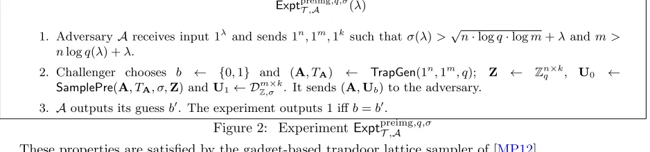
of trapdoor generation algorithms T = (TrapGen,SamplePre) is said to satisfy the (q, σ)-well-sampledness of preimage property if for any stateful PPT adversary A, there exists a negligible function negl(·) such that for allλ∈ N, q=q(λ), σ=σ(λ), prTpreimg,A ,q,σ(λ) = Pr[1←ExptTpreimg,A ,q,σ(λ)]≤1/2 + negl(λ), where ExptpreimgT,A ,q,σ(λ) is defined in Figure2.
ExptpreimgT,A ,q,σ(λ)
1. AdversaryAreceives input 1λand sends 1n,1m,1k such thatσ(λ)>√n·logq·logm+λand m >
nlogq(λ) +λ.
2. Challenger chooses b ← {0,1} and (A, TA) ← TrapGen(1n,1m, q); Z ← Znq×k, U0 ← SamplePre(A, TA, σ,Z) andU1← DZm,σ×k. It sends (A,Ub) to the adversary.
3. Aoutputs its guessb0. The experiment outputs 1 iffb=b0.
Figure 2: ExperimentExptpreimgT,A ,q,σ
These properties are satisfied by the gadget-based trapdoor lattice sampler of [MP12].
13Note that the pre-image sampling algorithm could be easily generalized to generate pre-images of matrices in
Znq×k (for
anyk) by independently runningSamplePrealgorithm on each column of the matrix. Throughout this work, we overload the notation by directly giving matricesU∈Znq×kas inputs to theSamplePrealgorithm.