IJCSMC, Vol. 3, Issue. 1, January 2014, pg.345 – 354 RESEARCH ARTICLE The Image Quality in Computer Tomography Using Curve-let Transform

(1)

345

Available Online atwww.ijcsmc.com

International Journal of Computer Science and Mobile Computing

A Monthly Journal of Computer Science and Information Technology

ISSN 2320–088X

IJCSMC, Vol. 3, Issue. 1, January 2014, pg.345 – 354

RESEARCH ARTICLE

The Image Quality in Computer Tomography

Using Curve-let Transform

M.Selvi

1

, J.Vanitha

2

, S.Yasotha

3

Student1, Assistant Professor2, Assistant Professor3 Dept. of CSE,

1

Sri Eshwar College of Engineering, Coimbatore, India

2

Sri Subramanya College Of Engineering, Palani, India

3

Sri Eshwar College of Engineering, Coimbatore, India

[email protected], [email protected], [email protected]

Abstract-The purpose of the ct-image de-noising is an important research topic both in image processing and biomedical

engineering. Independent component analysis (ica) is a statistical technique where the goal is to represent a set of random

variables as a linear transformation of statistically independent component variables. The curve let transform as a multiscale

transform has directional parameters occur at all scale, locations, and orientations. in this proposed a new model for ct

medical image de-noising, which is using independent component analysis and curve let transform. By this approach could

remove more noises and reserve more details, and the efficiency of our approach is better than traditional de-noising

approaches.

Keywords – Computer Tomography (CT); denoising Filters; image quality; radiation dose; curve let transform; Independent

Component Analysis

I. INTRODUCTION

The benefits of image processing is any form of Signal processing for which the input is an image Such as photography or

video frame; the output of Image processing may be either an image or a set of Characteristics or parameters related to the

image. Most image-processing techniques involve treating the image as a two-dimensional signal and applying standard

(2)

346

Image processing usually refers to digital image processing but optical and analog image Processing are also possible .The

article is about General techniques that apply to all of them. The Acquisition of image producing the input image in the first

place is referred to as imaging.

Computer Tomography(CT) [1]is a radiographic inspection method that generates a 3-D image of the inside of

improvement in tube technology, computer and hardware performanceshas led to an evolution of CT scanners, reducing the

acquisition scan times and improving the resolution. A first development of the traditional CT scanner is the spiral or helical

scanner.

It is based on the continuous patient motion through the gantry combined with the interrupted tube rotation. The name of this

scanner technology derives from the helical path traced out by the X-ray beam. The major advantage of helical scanning

compared with the traditional approach consists of its improved speed and spatial resolution.

II. RADITION DOSE AND IMAGE QUALITY

CT accounts for 47% of whole medical radiation, although it represents only 7% of total radiology examinations. Hence the

development of techniques for reducing the radiation dose becomes essential, particularly in pediatric application [2]. In

conventional radiography imaging, it is usually clear when overexposure has taken place. This is not true in CT, because the

amount of radiation adsorbed by the patient depends on many technical parameters, which can automatically be controlled by

CT scanners to balance the high image quality and the exposure dose.

Then it is possible that the difference between an adequate image and a high-quality image are not so immediately evident.

Unfortunately, as the radiation increases, the associated risk of cancer is increased, although this is extremely small. The

potential health risks associated with the radiation dose have motivated the American college of radiology to publish guidelines

to ensure that CT imaging protocols are optimized for the diagnostic image quality at the lowest radiation dose possible.

To bind the image quality to the radiation dose, a lot of dose descriptors were developed. The Computer Tomography Dose

Index, along with its variants, includes a set of standard parameters’ used to describe CT associated dose. It is a defined as the

integral of the dose distribution profile divided by the nominal slice thickness. Many technical factors contribute to the intensity

dose in CT.

Generally, in CT examinations, a high radiation dose results in high quality images. A lower dose leads to the increase in image

noise and results in unsharp images. This is more critical in low-contrast soft -tissue imaging like abdominal or liver CT. The

relationship between the image quality and the dose in CT is relatively complex, involving the interplay of a number of factors,

including noise, axial and longitudinal resolutions and slice width. Depending on the diagnostic task, these factors interact to

determine image sensitivity.

III. CT IMAGE NOISE

CT images are intrinsically noisy [3], and this poses significant challenges for image interpretation, particularly in the context of

low-dose and high-throughput data analysis. CT noise affects the visibility of low- contrast object. By using well-engineered CT

(3)

347

contributor to the total noise is the quantum noise, which represents the random variation in the attenuation coefficients of the

individual tissue voxels. In fact, it is possible that two voxels of the same tissue produce different CT values.

A possible approach to reduce the noise is the use of large voxels, absorb a lot of photons, assuming a more accurate

measurement of the attenuation coefficients. However, the use of large voxels increases blurring and limits the visibility

of fine details. Some image elaboration techniques allow one to significantly reduce the radiation dose without

compromising the image quality. These techniques work as filters, reducing random noise and enhancing structures. This way, it

is possible to obtain, at the same time , high quality images and low-dose radiation. Some image filters to reduce the noise

contribution were proposed. In a first step, the statistical properties of image noise in CT exams were investigated.

As evident in the literature, noise modeling and the way to reduce it are common problems in most imaging applications. In

many image processing applications, a suitable denoising phase is often required before any relevant information could be

extracted from analyzed images. This is particularly necessary when few images are available for analysis.

IV. NOISE REDUCTION

Noise reduction is the process of removing noise from Signal. Noise reduction techniques[4] are conceptually very similar

regardless of the signal being processed, however a priori knowledge of the characteristics of an expected a signal can

mean the implementations of these techniques vary greatly depending on the type of signal. All recording devices, both

analogue and digital, have traits which make them susceptible to noise. Noise can be random or white noise with no coherence

or coherent noise introduces by the device’s mechanism or processing algorithms.

In electronic recordings devices, a major form of noise is HISS caused by random electrons that, heavily influenced by heat

stray from their designated path. These stray electrons influence the voltage of the output signal and thus create detectable noise.

In the case of photographic film and magnetic tape, noise both visible and audible is introduced due to the grain structure of the

medium. In magnetic tape, the larger the grains of the magnetic particles usually ferric oxide or magnetite, the more prone the

medium are to noise. To compensate for this, larger areas of film or magnetic tape may be used to lower the noise to an

acceptable level.

To reduce the noise effect, different Low-pass filters have largely been used in medical image Analysis, but they have the

disadvantages to introduce Blurring edges. In fact, all smoothing filters, while smoothing out the noise, also remove high

frequency Edges features by degrading the localization and the Contrast. Therefore, it is necessary to balance the Trade- off

among noise suppression, image deblurring And edge detection To this aim, a low- pass filters combined With an edge

detector operator was proposed. In Particular, Gaussian, averaging and unsharpfilters were tested to smooth the noise, whereas

prewitt and sobel operators were used for edge identification. The experimental result showed that the combination of Gaussian

and prewitt offers best performances of the diffusion filter by increasing the action of the filter on the directions parallel to the

(4)

348

Fig 1. (a) Original CT image obtained with a high dose of radiation, (b) Emulated low-dose CT image obtained by

corrupting the high- dose CT image

Successively, a non lineardenoising technique has been tested, and its performances have been compared with the

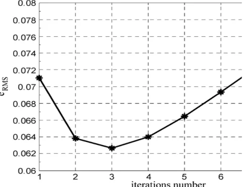
Gaussian-Prewitt filtering technique. Anisotropic diffusion is a selective and nonlinear filtering technique that improves image quality,

removing the noise while preserving and even enhancing details. The anisotropic diffusion processemploys the diffusion

coefficients to determine the amount of smoothing that should be applied to each pixel of the image

It is possible to note that the local menu. In fact Even if the global noise mean is zero, locally the mean is Usually non zero.

Obtaining four K values for each diffusion Function.Thediffusion does not take into account the edge Direction. In fact ,they

(5)

349

V. MATERIALS AND METHODS

A.Gaussian Filter and Prewitt Operators

The one- dimensional Gaussian filter has an impulse response given by

Or with the standard deviation as parameter.

In two dimensions, it is the product of two such gaussians,one per directions.

Where x is the distance from the origin in thehorizontal axis,y is the distance from the origin in the vertical axis, and σ is the

standard deviation of the Gaussian distribution.

The Gaussian filter is non-causal which means the filter window is symmetric about the origin. This is usually of no

consequence for most applications. In real-time systems, a delay is incurred because incoming samples need to fill the filter

window before the filter can be applied to the signal.

Gaussian smoothing

Gaussian smoothing is often applied because the noise or the nature of the object might be of a Gaussian probable form. A two

dimensional Gaussian Kernel defined by its kernesize and standard deviation(s). Below are the formulas for 1D and 2D

Gaussian filter shown SDx and SDy are the standard deviation for the x and y directions respectively.

The Gaussian filter works like the parametric LP filter but with the difference that larger kernels can be chosen. Below a

Gaussian filter is shown in 2D top view with horizontal and vertical cross sections and also in 3D view. The Gaussian function

shown has a standard deviation of 10x10 and a kernel size of 35x35 pixels.

Smoothing Filters

Smoothing filters are also called low-pass filters because they let low frequency components pass and reduce the high frequency

(6)

350

Low-pass filtering in effect blurs the image and removes speckles of high frequent noise. Larger masks will result in more

blurring effect. To avoid a general amplification or damping of the data the sum of the filter coefficients should be 1.0In

practice the low-pass filter can be used for creating high pass filters by subtracting the filtered result from the original image or

by some other combination of the input image and the filtered result as described in the. "Unsharp Masking" section.

B.Anisotropic Diffusion

In image processing and computer vision, anisotropic diffusion, also called Perona–Malik diffusion, is a technique aiming at

reducing image noise without removing significant parts of the image content, typically edges, lines or other details that are

important for the interpretation of the image.Anisotropic diffusion resembles the process that creates a scale-space, where an

image generates a parameterized family of successively more and more blurred images based on a diffusion process. Each of the

resulting images in this family is given as a convolution between the image and a 2D isotropic Gaussian filter, where the width

of the filter increases with the parameter. This diffusion process is a linear and space-invariant transformation of the original

image. Anisotropic diffusion is a generalization of this diffusion it produces a family of parameterized images, but each

resulting image is a combination between the original image and a filter that depends on the local content of the original image.

As a consequence, anisotropic diffusion is a non-linear and space-variant transformation of the original image.

In its original formulation, presented by Perona and Malik in 1987, the space-variant filter is in fact isotropic but depends on the

image content such that it approximates an impulse function close to edges and other structures that should be preserved in the

image over the different levels of the resulting scale-space. This formulation was referred to as anisotropic diffusion by Perona

and Malik even though the locally adapted filters are isotropic, but it has also been referred to as inhomogeneous and nonlinear

diffusion or Perona-Malik diffusion by other authors. A more general formulation allows the locally adapted filter to be truly

anisotropic close to linear structures such as edges or lines: it has an orientation given by the structure such that it is elongated

along the structure and narrow across [5]. As a consequence, the resulting images reserve linear structures while at the same

time smoothing is made along these structures. Both these cases can be described by a generalization of the usual diffusion

equation where the diffusion coefficient, instead of being a constant scalar, is a function of image position and assumes a matrix

(or tensor) value.

Although the resulting family of images can be described as a combination between the original image and space-variant

filters, the locally adapted filter and its combination with the image do not have to be realized in practice. Anisotropic

diffusion is normally implemented by means of an approximation of the generalized diffusion equation: each new image in

the family is computed by applying this equation to the previous image. Consequently, anisotropic diffusion is an iterative

process where a relatively simple set of computation are used to compute each successive image in the family and this

process is continued until a sufficient degree of smoothing is obtained.

(7)

351

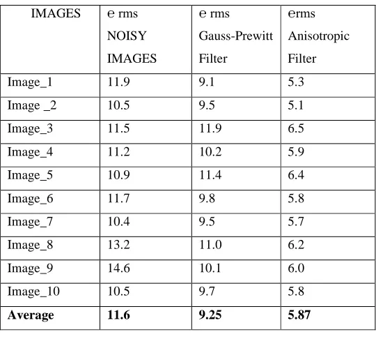
Denotes the gradient, is the divergence operator and c(x,y,t) is the diffusion coefficient

Table 1.erms without curvelet filter

An image de-noising model by integrating anisotropic diffusion with USFFT curve let transform was implemented, which

combined the strong point of curve let transform with anisotropic diffusion (P-M Diffuse on).

By choosing appropriate gradient threshold K through p-norms and carrying out the P-M diffusion process depend on the

different scale matrixes of curve let coefficient of the image from curve let transform iterations, as a result, the improved model

made it possible to carry out the new P-M diffusion de-noising process based on multi-scale analysis of the image[6] . The

experiment results have demonstrated that the model can avert the stair-casing effect in the traditional P-M diffusion effectively

and keep the textures and details of image better.

VI. PERFORMANCE EVALUATION

By calculating the erms value in the existing system by using wavelet transforms for the low dose radiation images. The result

of them isOnly 5%.To over come the existing system problem we are implementing the curve let transform towards through in

this method by using this method the erms will decrease its error in the low radiation and we get a clear and neat output will

been shown below.

The Curve let transform is a higher dimensional Generalization of the wavelet transform designed to represent Images at

different scales and different angles. Curved Singularities can be well approximated with very few Coefficients and in a non-

IMAGES ℮ rms

NOISY

IMAGES

℮ rms

Gauss-Prewitt

Filter

℮rms

Anisotropic

Filter

Image_1 11.9 9.1 5.3

Image _2 10.5 9.5 5.1

Image_3 11.5 11.9 6.5

Image_4 11.2 10.2 5.9

Image_5 10.9 11.4 6.4

Image_6 11.7 9.8 5.8

Image_7 10.4 9.5 5.7

Image_8 13.2 11.0 6.2

Image_9 14.6 10.1 6.0

Image_10 10.5 9.7 5.8

(8)

352

adaptive manner. Hence the name curve lets. Curve lets remain coherent waveforms under the action of the wave equation in a

smooth medium.

If

at all points on , then implies

.

Let .

Then:

We now briefly return to the continuum viewpoint suppose we set an initial goal to produce a decomposition using the

multiscale ridge let pyramid. The hope is that this would allow us to use thin “brushstrokes” to reconstruct the image,

with all gths and widths available to us. In particular, this would seem allow us to trace sharp edges precisely using a

few elongated elements with very narrow widths.

Ever since donoho’s curve let based thresholding approaches was published in 1995, there was a surge in the de noising

projects being published. Although donoho’s concept was not revolutionary, his method did not require tracking or correlation

of the wavelet maxima and minima across the different scales as proposed. Thus there was a renewed interest in curve let based

denosing techniques demonstrated a simple approach to a difficult problem.

image Erms

noisy

image

Erms

Gaussian-prewitt

filters

Erms

anisotropic

filters

Erms

CurveLet

Img 1 12.6 16.68 14.95 10.64

Img 2 11.9 20.60 12.95 9.47

Img 3 13.7 16.68 1495 6.74

Img 4 12.7 14.27 12.97 9.30

Img 5 13.9 19.23 15.47 8.45

(9)

353

Img 7 12.6 13.03 13.83 7.26

Img 8 14.6 23.92 24.64 7.38

Img 9 13.4 14.54 10.88 7.54

Img10 13.5 11.62 11.92 9.09

Average 13.14 16.49 14.35 8.32

Table 2.erms value with curve let values

VII. CONCLUSION

This paper proposes a new model for CT medical image de noising, which is using independent component analysis and curve

let transform. Firstly, a random matrix was produce to separate the CT image into a separated image into a separated image for

estimate. Then curve let transform was applied to optimize the coefficients .At last, the inverse of the curve let transform was

applied for image reconstruction. The de-noising image has a higher value of SNR and a lower value of MSE. This approach

could remove more noises and reserve more details. Some image filters to reduce the noise contribution were proposed.

The Gaussian blur is a type of image-blurring filters that uses a Gaussian function (which also expresses the normal distribution

in statistics) for calculating the transformation to apply to each pixel in the image. The equation of a Gaussian function in one

dimension is

intwo dimensions, it is the product of two such Gaussians, one in each dimension:

In particular, a combination of Gaussian and Prewitt filters was initially tested, obtaining a RMS of 10%. Successively, a

filtering technique based on anisotropic diffusion was applied. Several simulations have been carried out to choose the best filter

parameters. This way, it has been possible to decrease the relative error to about 6%. In future, investigations on the use of the

independent component analysis and curve let transform to optimize 3-D medical image processing are processed. This

approach could remove more noises and reserve more details, and the efficiency of our approach is better than other traditional

de-noising approaches. In future, investigations on the use of the independent component analysis and curve let transform to

optimize 3-D medical image processing are processed. This approach could remove more noises and reserve more details, and

the efficiency of our approach is better than other traditional de-noising approaches.

REFERENCES

[1] C. J. Garvey and R. Hanlon, “Computed tomography in clinical practice,” BMJ, vol. 324, no. 7345, pp. 1077-1080, May 2002

[2] M. Prokop, M. Galanski, A. J. van der Molen, and C. Schaefer-Prokop,Spiral and Multislice Computed Tomography of the Body. Stuttgart, NY:Thieme, 2003.

(10)

354

[4] S. Nam, H. J. Kim, J. Jung, H. M. Cho, and C. L. Le, “Quantitative Imaging with low-dose CT in PET/CT system,” in Conf. Rec. IEEE Nucl. Sci., 2007, pp. 3436-3439

[5] M. Kachelrie and W. A. Kalender, “Presampling, algorithm, and noise: Considerations for CT in particular for medical imaging in general,” Med. Phys., vol. 32, no. 5, pp. 1321-1334, May 2005.

[6] P. Gravel, G. Beaudoin, and J. A. De Guise, “A method for modeling noise in medical images,” IEEE Trans. Med. Imag., vol. 23, no. 10, pp.1221-1232, Oct. 2004.

[7] D. L. Donoho and M. R. Duncan, “Digital curve let transform: Strategy,implementation and experiments,” Proc. SPIE, vol. 4056, pp. 12–29, 2005

[8] Starck, J. L.; Candes, E. J. & Donoho, D. L. (2000). The curve let transform for image denosing, IEEE Transactions on Image Processing, vol. 11, pp. 670–684, 2000

[9] Choi, M.; Kim, R. Y. & Kim, M. G. (2004). The curve let transform for image fusion, Proc ISPRS Congress, Istanbul, 2004

[10] Candes, E. J. & Donoho, D. L. (2000). Curvelets—A surprisingly effective non- adaptive representation for objects with Edges, Vanderbilt University Press, Nashville, TN, 2000.

Authors Profile

M. SELVI pursuing M.E (Computer Science and Engineering) Second Year in Sri Eshwar college of Engineering, Coimbatore. She has completed her B.E in Maharaja Engineering college in 2012.Her area of interest is Wireless Sensor Network.

VANITHA.J has done M.E in Computer Science from PSNA in 2011. She has done her B.E in Computer Science from Sri Subramanya College of Engg and Tech. She is currently working as Assistant Professor at College of Sri Subramanya College of Engg and Tech Palani. Her Current research areas include Image Processing.