The Potential of Active Contour Models in Extracting
Roads from Mobile Laser Scanning Data
Pankaj Kumar1,†*, Paul Lewis2and Tim McCarthy2,
1 Geomatics Division, Centre Tecnològic de Telecomunicacions de Catalunya (CTTC/CERCA), Castelldefels,
Barcelona, Spain
2 National Centre for Geocomputation, Maynooth University, Co. Kildare, Ireland; [email protected] (P.L.);
[email protected] (T.M.)
* Correspondence: [email protected]; Tel.: +34-936-452-900.
† Current address: Geomatics Division, Centre Tecnològic de Telecomunicacions de Catalunya (CTTC/CERCA), Castelldefels, Barcelona, Spain
Abstract:Active contour models present a robust segmentation approach which make efficient use of specific information about objects in the input data rather than processing all the data. They have been widely used in many applications including image segmentation, object boundary localisation, motion tracking, shape modelling, stereo matching and object reconstruction. In this paper, we investigate the potential of active contour models in extracting roads from Mobile Laser Scanning (MLS) data. The categorisation of active contours based on their mathematical representation and implementation are discussed in detail. We discuss an integrated version in which active contour models are combined to overcome their limitations. We review various active contour based methodologies which have been developed to extract roads and other features from LiDAR and digital imaging datasets. We present a small case study in which an integrated version of active contour models is applied to automatically extract road edges from MLS dataset. An accurate extraction of left and right edges from the tested road section validates the use of active contour models. The present study provides a valuable insight on the potential of active contours for extracting roads and other infrastructures from 3D LiDAR point cloud data.
Keywords:active contour models, LiDAR, segmentation, road edges
1. Introduction
Light Detection And Ranging (LiDAR) enables 3D modelling of real world environment by measuring the time of return of an emitted light pulses. The information obtained through laser scanning systems, which use LiDAR technology, have application in road safety, urban planning, flood plain, glacier and avalanche mapping, bathymetry, geomorphology, forest survey, bridge and transmission line detection [1–3]. They provide several benefits over conventional sources of data acqusition in terms of accuracy, resolution, attributes and automation [4]. The applicability of laser scanning systems continue to prove their worth in mapping due to their ability to provide georeferenced set of dense LiDAR point cloud data [5–7]. LiDAR data records a number of attributes including elevation, intensity, pulse width, range and multiple echo, all of which can be used for extracting information about real world environment. The methods developed for segmenting LiDAR data are mostly based on the identification of planar or smooth surfaces and the classification of point cloud data based on its attributes [8].
Active contour models present a robust segmentation approach which make efficient use of specific information available about objects in the input data rather than processing all the data [9]. The concept of active contour was first introduced by [10] and has been widely used for image segmentation [11,12]. In this paper, we examine the potential of active contour models in extracting roads from Mobile Laser Scanning (MLS) data. In Section2, we discuss active contours and their categorisation in detail. Section3reviews various approaches based on active contour models which have been
developed for extracting roads and other objects from LiDAR and digital imaging datasets. In Section 4, we present a case study in which an integrated version of active contour models is applied to extract road edges from MLS dataset. In Section5, the road edge extraction results are discussed and finally, the conclusions are drawn in Section6.
2. Active Contour Models
Active contour models provide an efficient framework for object delineation from the input data. They can be distinguised as parametric and geometric models [13]. The difference between the two versions is how the contour is defined and behaves. The parametric active contour is represented explicitly as a controlled spline curve that is implemented based on energy computations. The geometric active contour is represented implicitly as a level set and is evolved based on geometric computations. In the following sections, we describe parametric and geometric active contour models in detail.
2.1. Parametric Active Contour Model
The parametric active contour, or snake, is defined as an energy minimising parametrised curve within a 2D image domain that moves towards a desired object boundary under the influence of an internal energy within the curve itself and an external energy derived from the image data [10]. The internal energy is applied to the curve which controls the curve’s elasticity and rigidity, while the external energy attracts the snake curve towards the object boundary. The movement of the snake curve is controlled through balancing the internal and external energy terms until an energy minimisation condition is met. When the snake’s energy function reaches a minimum, it converges to the object boundary.
The snake is defined parametrically in the(x,y)plane of an image as
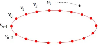
v(s) = [x(s),y(s)], (1) wherex(s),y(s)are coordinates along the snake curve andsis the normalised arc length. The curvev(s)is represented by a set of control pointsv0,v1...vn−1and is linearly obtained by joining each control point as shown in Figure1.
Figure 1.Snake curve initialised in the form of parametric ellipse.
The snake’s energy function can be described as
Esnake= n−1 Z
0
Esnake(v(s))ds. (2)
The energy function constituting the internal and external energy terms is described as
Esnake= n−1 Z
0
(Eint(v(s)) +Eext(v(s)))ds, (3)
The internal energy controls the snake curve’s elasticity and stiffness properties. The internal energy functionEintcan be written as
Eint= 1 2(α(s)|
dv ds|
2+ β(s)|d
2v ds2|
2), (4)
whereα(s)andβ(s)are weight parameters. Equation4is composed of two terms, a first-order term designed to hold the curve together and a second-order term designed to keep the curve from bending. Theαweight parameter controls elasticity while theβweight parameter controls stiffness in the snake curve [14].
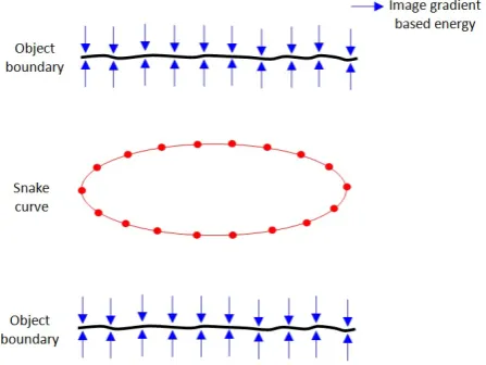
The external energy creates a gradient image that attracts the snake curve toward the object boundaries as shown in Figure2.
Figure 2.Snake curve initialised on gradient image of object boundaries.
The image gradient based external energy is described as
Eext=−κ|Of(v(s))|2, (5)
whereκis a weighting parameter andOf is the gradient image of object boundaries, f.
For the snake curve to converge on the object boundary, the snake’s energy function,Esnakein Equation3, should be minimised. To minimise the energy function, the snake curve must satisfy the Euler condition as [15]
d ds(α(s)
dv ds)−
d2 ds2(β(s)
d2v
ds2)−OEext(v(s)) =0, (6) wherevsis a derivative ofvwith respect tos. To find a solution to Equation6, the snake is made dynamic by treatingvas a function of timetwhich leads to
∂v(s,t) ∂t =
∂
∂s(α(s) ∂v(s,t)
∂s )− ∂2 ∂s2(β(s)
∂2v(s,t)
∂s2 )−OEext(v(s,t)). (7) A solution to Equation7is found by discretising it and solving the discrete system iteratively
[16]. When the term ∂v(s,t)
∂t approaches 0, the snake’s energy function reaches its minimum and is expected to have converged on the object boundary.
Figure 3.Parametric active contour model applied to an object with a concave boundary [16].
Several methods have been developed to overcome these limitations in the parametric active contour model [18]. In the following sections, we discuss modified versions of the parametric active contour model which have been developed to overcome these limitations.
2.1.1. Balloon Model
To overcome the snake initialisation limitation, [19] introduced a balloon concept in the parametric active contour model in which an additional energy is added to the external energy term which pushes a snake curve towards an object boundary. In the balloon model, the snake curve behaves like a balloon which is inflated by the additional energy. The balloon energy acts in the normal direction to a point on the curve which makes the behaviour of the snake curve more dynamic. The modified external energy term in the parametric active contour model can be described as
Eext=κballoonn(s)−κ|Of(v(s))|2 (8) whereκballoonis the weight parameter for the balloon energy andn(s)is the unit vector normal to the snake curve at pointv(s). If the sign ofκballoonis negative, it will have a deflating effect instead of an inflating effect over the snake curve.
The balloon energy pushes the snake curve towards object boundaries while the image gradient based energy attracts the snake curve toward the object boundaries, as shown in Figure4.
Figure 4.Balloon external energy added to the snake curve.
balloon energy. This can have the added benefit of overcoming spurious noise in the data while detecting the object boundaries [15].
The primary advantage of the balloon model is that it increases the movement range of the snake curve towards the object boundaries. It overcomes the snake curve initialisation drawback in the traditional parametric active contour model but it does not provide a solution for the concave boundary convergence problem. The value of balloon energy is also dependent on the image gradient energy and noise in the data.
2.1.2. GVF Model
[20] introduced a Gradient Vector Flow (GVF) external energy in the parametric active contour model in an attempt to detect the concave boundaries. It is based on diffused gradient vectors of the object boundaries. The GVF energy is described as the energy fieldV(x,y) = (u(x,y),v(x,y)), where uandvare its vector components in the(x,y)plane of an image. It minimises an energy function
E= Z Z
µ(u2x+u2y+v2x+vy2) +|Of|2|V−Of|2dxdy. (9) Noise in the data can prohibit the GVF energy from being calculated effectively. To control the impact of this noise, a regularisation parameter,µ, is used to balance the first term,µ(u2x+u2y+v2x+v2y) and the second term,|Of|2|V−Of|2of the Equation9. An increased noise in the image will require a higher value forµ. WhenOf is small or negligible, the energy function is dominated by the first term which is a sum of the squares of partial derivatives of the vector components. WhenOf is large, the second term dominates and minimises the energy function, whenV =Of. It results in a smoothly varying energy being produced over a homogeneous image region while not affecting the gradient energy along the object boundary.
The GVF energy is obtained by solving the following Euler equations [16]
µO2u−(fx2+ fy2)(u−fx) =0, (10)
µO2v−(fx2+fy2)(v− fy) =0, (11) whereO2is a laplacian operator and f
x,fyare the gradient components along theXandYaxis of the image. Equations10and11are solved by treatinguandvas functions of timetsuch that
ut(x,y,t) =µO2u(x,y,t)−(fx(x,y)2+fy(x,y)2)(u(x,y,t)− fx(x,y)), (12)
vt(x,y,t) =µO2v(x,y,t)−(fx(x,y)2+ fy(x,y)2)(v(x,y,t)− fy(x,y)). (13) Equations12and13are known as generalised diffusion equations [16]. After estimating the value ofV(x,y,t), the external energy term,OEext(v(s,t)), in Equation7is replaced giving us
∂v(s,t) ∂t =
∂
∂s(α(s) ∂v(s,t)
∂s )− ∂2 ∂s2(β(s)
∂2v(s,t)
∂s2 ) +V. (14)
The GVF energy attracts the snake curve toward the object boundaries, as shown in Figure5. The diffused energy allows the snake curve to detect the concave boundaries [16], shown in Figure6.
Figure 5.Snake curve initialised on GVF image of object boundaries.
Figure 6.GVF based parametric active contour model applied to an object with a concave boundary [16].
2.1.3. Integrated Model
We developed an integrated model in which the balloon and GVF based parametric active contour models are combined. In the integrated model, the balloon energy pushes the snake curve and the GVF energy attracts the snake curve toward the object boundaries, as shown in Figure7.
This is useful in the case where there is a relatively large distance between the initial snake and the object boundaries. The use of balloon energy increases the movement range of the snake curve while the GVF energy allows the snake curve to detect the object boundaries more efficiently. In this way, the integrated model can be applied to overcome both the limitations in the traditional parametric active contour model.
2.2. Geometric Active Contour Model
The geometric active contour model is based on a level-set and curve-evolution theory [22,23]. The primary advantage of the geometric active model is that it does not require any parameters for its implementation. A geometric curve is represented implicitly as a level-set and is evolved based on geometric computations, with its speed locally dependent on the image data [15]. The level-set refers to a set of point variables for which their function is equal to some constant value. For example, the level-set of the variables(x,y,z)can be the spherex2+y2+z2=r2, with centre (0,0,0) and radiusr [24].
Figure 7.Balloon energy pushes the snake curve and GVF energy attracts the snake curve toward the object boundaries.
Figure 8.Geometric active contour model.
∂ψ
∂t =c(k+V0)|Oψ|, (15)
wherecis given by
c= 1
1+|O(Gσ∗I)|
(16)
and is the potential energy derived from the input image,I. This parameter serves as the stopping term for the curve at the object boundary. The termO(Gσ∗I)is the gradient of the Gaussian blurred
image with standard deviation of the Gaussian distribution,σ. kis curvature of the curve, which makes it smoother,V0is a constant which has the effect of controlling the shrinking or expansion of the curve andOψis a gradient of the level-set,ψ. The termc(k+V0)determines the speed with which the curve evolves along its normal direction.
The geometric curve does not stop at weak or indistinct boundary points due to its evolution speed but continues its movement with little or no energy drawing it back [13]. To overcome this problem, an extra term can be added to Equation15as follows
∂ψ
This additional stopping termOcOψis used to pull back the curve in case it overpasses a weak object boundary.
The advantage of using the geometric active contour model is its ability to change a curve’s topology in accordance with the shape of the object during the curve evolution process. This can be useful in object tracking and motion detection applications. The geometric active contour model is generally not useful for noisy data where the evolved curve can be accompanied by topological inconsistencies [15]. The implementation of the geometric active contour model is based on geometric computations which results in it being a computationally expensive process [18]. In the next section, various approaches based on active contour models have been reviewed for extracting features from digital imaging and LiDAR datasets.
3. Related Work
The concept of active contours have been extensively studied to develop several improved models which include Generalized Gradient Vector Flow (GGVF) Snake [25], region-based active contours [26], Curvature Vector Flow (CVF) Snake [27], Geodesic GVF / GGVF Snake [28] and Magnetostatic Active Contour (MAC) Model [29]. The active contours have been widely used to develop methodologies for extracting buildings, coastlines and other features from high resolution digital images. [30] extended the concept of traditional snake to twin snakes for extracting linear features with two boundaries from high resolution digital imagery. An additional energy term was introduced in the snake’s energy function which formulated the attraction force in between the twin snake curves for detecting two parallel linear boundaries. [31] used a wavelet based parametric active contour model for detecting coastlines from satellite imagery. The wavelet transform was used to determine high gradient values in the images filtered at multiple scales. An active contour model was applied over the image at the coarsest scale. The final snake curve obtained at the coarsest scale was used to initiate the snake curve at next coarsest scale and this process was repeated until the original scale of the image was reached. [32] presented an improved snake model for detecting buildings from high resolution aerial images. Their model was focussed on utilizing the radiometric and geometrical properties of buildings for modifying the selection criteria of initial seeds and the external energy function. [33] developed a radial casting approach to initialise the snake curve for extracting building features from high resolution Quickbird imagery. In their method, a single seed point was placed at the approximate centre of each building object. The snake points were then generated in accordance with the radial lines projected outwards at various angular intervals from the centre seed point. [34] presented a new method for building boundary extraction from high resolution aerial images. Their method was based on region-based geometric active contour model in which building boundaries were detected by introducing certain training points in their vicinity. Finally, the detected building boundaries were generalized to obtain their regular shape. [35] developed an approach based on localized region-based geometric active contours for multitemporal monitoring of urban trees in a series of high resolution aerial images. In their approach, contours were initialized based on image fitting procedure and tree crown regions were identified using a localized data energy term. In the multitemporal analysis, a priori information was incorporated by initialising the contour in each image based on previously optimized contours.
the road. [38] developed a framework for semi-automatic highway extraction from high resolution aerial orthophotographs using geometric active contour model. In their approach, the boundary and region-based information of highway features was incorporated as constraint in the model for extraction procedure. [39] used a self-adaptive template matching method to provide the initialisation to the Least Square B-spline (LSB) snake model for extracting road objects from high resolution satellite imagery. In the template matching method, various templates of road width and luminance attribute were matched with manually selected points in the image. The result with maximum matching was used to initialise the snake for extracting road features.
Apart from digital images, few methods based on active contour models have also been developed for extracting features from LiDAR data. [40] proposed an approach for surface reconstruction from LiDAR data. In their algorithm, a surface was grown from an initial seed point in the LiDAR data based on the extended snake model. The internal energy was provided by placing a constraint on the angle in between the normal vectors of two adjacent planar patches in order to maintain the smoothness of a reconstructed surface. The external energy was modelled as a function of distance from the LiDAR points to the corresponding planar patch. [41] applied a snake model to extract the road network for integrating and matching, 2D Digital Landscape Model (DLM) derived from 2D vector data and Digital Terrrain Model (DTM) generated from airborne LiDAR data. In their approach, the snake curve was initialised near the road feature using existing vector data, stored as a polyline, while the external energy terms were derived from intensity, elevation and surface roughness based images generated from the LiDAR data. The energy of the snake contour was minimised which led to its convergence to the road network. The extracted road network information was then used to integrate the two datasets. Later, they extended their work to include building and bridge information in order to support the road extraction process using the snake model [42]. [18] proposed an improved snake model for extracting buildings from aerial images and LiDAR data. The initial estimation of building edges was carried out by applying a threshold to the Normalised Digital Surface Model (NDSM). The snake model was implemented by deriving the external energy terms based on intensity and altitude variances of the snake curve points with their neighbourhood points. [43] described a method for extracting roads from a large scale 3D point cloud data merged from aerial and terrestrial laser scanning of an urban environment. An initial approximation of the road network in the point cloud data was made using 2D map and then the road network was divided into independent patches to make the process computationally efficient. In each patch, an active contour model was applied by estimating the elevation based attractor function as an external energy of the snake curve to find the kerbs in the urban road sections. [44] presented an approach for roof modeling from airborne laser scanning data based on level set function. In their approach, the energy function of multiphase level set was used to segment roof plans into multiple homogeneous regions with similar normal vectors. Finally, the roof segments and their topological relations were used to reconstruct 3D roof model.
4. Case Study
We conducted this experimental study to demonstrate the ability of active contour models in extracting road features from MLS dataset. We developed an automated approach in which integrated version of parametric active contour models is applied to extract left and right edges from MLS data [4]. The implementation of parametric active contour model is less computationally expensive in comparison with the geometric active contour model and it gives structured control on elasticity and stiffness properties of the snake.
In our developed approach, the input data sections are selected with some overlap between them which allows to batch process consecutive and overlapped road sections [45]. We use elevation and intensity attributes of the LiDAR data. These point cloud attributes are converted into 2.5D raster surfaces using point thinning and natural neighbourhood interpolation method [46]. The cell sizec parameter, required to generate the raster surfaces is selected empirically based on an experimental analysis [45]. A slope raster surface is generated from the elevation surface. The GVF external energy terms are computed as diffused energy field of the gradient vectors of the object boundaries from the raster surfaces. To compute the GVF energy, the object boundaries are determined from the slope and intensity raster surfaces respectively through the consecutive use of hierarchical thresholding and Canny edge detection [15]. The GVF external energy terms are estimated by iteratively diffusing gradient vector values of the object boundaries. The weight of the slope and intensity based GVF energy terms are set with theκslopeandκintparameters respectively. The balloon energy is included in the external energy by providing a weight to the normal unit vector of the snake curve points with theκballoonparameter. The values of the weight parameters for the GVF and balloon energy terms are estimated empirically based on experimental analysis and then same values were applied for each road section [47]. Internal energy is provided to the snake curve by adjusting its elasticity and stiffness properties withαandβweight parameters while the step size of the snake curve is controlled with aγ weight parameter. The topology of the left and right edges in the road sections do not vary much, thus, same internal energy weight parameters can be used for each road section. Their values are estimated empirically based on experimental analysis [47].
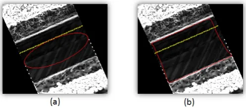
The snake curve is automatically initialised over a 2.5D raster surface using the navigation track of the mobile van along the road section. The snake curve moves under the influence of the internal and external energy terms. It approaches the minimum energy state during an iterative process and converges to the road edges. An example of initial and final position of the snake curve is shown in Figure9.
Figure 9.An (a) initial and (b) final position of the snake curve.
them. For more information about the developed road edge extraction approach, readers can refer to [4].
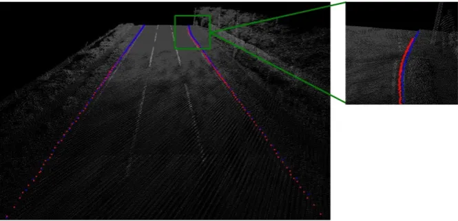
We tested our automated road edge extraction approach on 50m section of road which consisted of a grass-soil edge along its left side and a kerb edge along its right side. This road section was selected to validate the robustness of our approach in extracting distinct sets of edges. The processed dataset for the road section was acquired using StreetMapper MLS system in County Nottinghamshire, UK [48]. To process the road section, we used 6 sets of 30m×10m×5m section of LiDAR data and 6 sets of 10m section of navigation data. The road edge extraction approach was applied to the road section with an empirically selected parameters asc=0.06m2,κslope =4,κslope=2,κballoon=1,α=9,β=0.001 andγ=3. The left and right edges in the selected road section were also manually digitised in order to make comparison with the edges extracted through the automated approach. The automatically extracted 3D edges are represented in red while the manually digitised 3D edges are represented in blue in the road section as shown in Figure10.
Figure 10.The automatically extracted 3D edges are represented in red and the manually digitised 3D edges are represented in blue in the 50m road section. The inset picture of right edge show some of the points in detail.
In the next section, we validate the road edge extraction results and discuss them.
5. Results & Discussion
We validated the automatically extracted 3D edges in the road section by estimating their orthogonal proximity from the manually digitised 3D edges. These orthogonal values were estimated based on the navigation points selected at some interval along the road section [47]. The positive or negative values indicate the inside or outside position of the extracted road edge points with respect to the digitised road edge points. Box plots for the accuracy values of these extracted left and right edges in the road section are shown in Figure11.
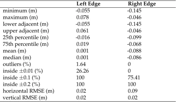
We also carried out statistical analyses of these accuracy values for the extracted edges as shown in Table1.
Figure 11.Box plot for the accuracy values of the automatically extracted left and right edges in the road section.
Table 1.Statistical analysis of the accuracy values of the automatically extracted left and right edges in the road section.
Left Edge Right Edge
minimum (m) -0.055 -0.145
maximum (m) 0.078 -0.046
lower adjacent (m) -0.055 -0.145
upper adjacent (m) 0.061 -0.046
25th percentile (m) -0.016 -0.099
75th percentile (m) 0.019 -0.068
mean (m) 0.001 -0.088
median (m) 0.001 -0.086
outliers (%) 1.64 0
inside±0.01 (%) 26.26 0
inside±0.1 (%) 100 75.41
inside±0.2 (%) 100 100
horizontal RMSE (m) 0.02 0.09
vertical RMSE (m) 0.02 0.02
tolerances were higher for the left edge. The left edge accuracy values were found to be fully inside
±0.1m while the right edge accuracy values were fully inside±0.2m.
[49] reported an average horizontal and vertical root mean square error (RMSE) values of 0.08 and 0.02m respectively, for the kerb edges extracted from MLS data. In comparison, our approach extracted the kerb edges along right side of the road section with horizontal and vertical RMSE values of 0.09 and 0.02m respectively. This accuracy level can be further improved with the use of a reflectance attribute which is a representation of the normalised intensity values. The availability of a pulse width attribute in the acquired dataset will also provide us to use their values to generate an additional GVF energy. This will improve the road edge extraction accuracy as pulse width values can be used to distinguish the road surface from its edges more efficiently.
6. Conclusion
integrated version of parametric active contour models was applied to automatically extract left and right edges from MLS dataset. In the integrated version, the active contour models are combined so as to overcome the limitations existing in them. The developed road edge extraction approach is based on the assumption that the LiDAR elevation and intensity attributes can be used to distinguish the road surface from the grass-soil and the kerb edges. The successful extraction of road edges validates the potential of active contour models in extracting features from MLS data. We intend to investigate the applicability of geometric active contour model in extracting features from LiDAR data. This could be advantageous as it will remove the requirement for weighting various input parameters.
Acknowledgments:Research presented in this paper was initially funded by the Irish Research Council Enterprise Partnership scheme and Strategic Research Cluster grant 07/SRC/I1168 awarded by Science Foundation Ireland under the National Development Plan. This research also recieved support through Science Foundation Ireland grant 13/IF/I2782. The authors also acknowledge the 3D Laser Mapping company for providing the Streetmapper MLS data.
Author Contributions:Pankaj Kumar collaborated with Paul Lewis in developing the approach and performing the experiments. Tim McCarthy provided technical advice at all stages. All authors contributed equally in preparing this manuscript.
Conflicts of Interest:The authors declare no conflict of interest.
Abbreviations
The following abbreviations are used in this manuscript:
MLS Mobile Laser Scanning LiDAR Light Detection and Ranging GVF Gradient Vector Flow
GGVF Generalized Gradient Vector Flow CVF Curvature Vector Flow
MAC Magnetostatic Active Contour DLM Digital Landscape Model DTM Digital Terrain Model
NDSM Normalized Digital Surface Model
References
1. Burtch, R. LiDAR principles and applications. Proceedings of Imagine Conference, Traverse City, 29 April - 1 May2002, pp. 1–13.
2. Mallet, C.; Bretar, F. Full-waveform topographic LiDAR: state-of-the-art. ISPRS Journal of Photogrammetry and Remote Sensing2009,64, 1–16.
3. Lohani, B. Airborne altimetry: principle, data collection, processing and applications. Available at http://home.iitk.ac.in/˜blohani/LiDAR_Tutorial/Airborne_AltimetricLidar_Tutorial.htm (Accessed: 12.01.2016), 2016.
4. Kumar, P.; McElhinney, C.P.; Lewis, P.; McCarthy, T. An automated algorithm for extracting road edges from terrestrial mobile LiDAR data. ISPRS Journal of Photogrammetry and Remote Sensing2013,85, 44–55. 5. Petrie, G.; Toth, C.K. Introduction to laser ranging, profiling and scanning. InTopographic laser ranging and
scanning: principles and processing; Shan, J.; Toth, C.K., Eds.; Taylor & Francis Group: Boca Raton, US, 2008. 6. Kumar, P.; McElhinney, C.P.; Lewis, P.; McCarthy, T. Automated road markings extraction from mobile laser scanning data.International Journal of Applied Earth Observation and Geoinformation2014,32, 125–137. 7. Kumar, P.; Lewis, P.; McElhinney, C.P.; Rahman, A.A. An algorithm for automated estimation of road
roughness from mobile laser scanning data.The Photogrammetric Record2015,30, 30–45.
8. Vosselman, G. Advanced point cloud processing. Proceedings of Photogrammetric Week, Stuttgart, 7-11 September2009, pp. 137–146.
9. Blake, A.; Isard, M.Active Contours; First edition, Springer, London, 1998.
11. Lundervold, A.; Storvik, G. Segmentation of brain parenchyma and cerebrospinal fluid in multispectral magnetic resonance images. IEEE transactions on medical imaging1995,14, 339–349.
12. Panah, M.; Javidi, B. Segmentation of 3D holographic images using jointly distributed region snake. Optics Express2006,14, 5143–5153.
13. Xu, C.; Yezzi, A.; Prince, J.L. On the relationship between parametric and geometric active contours. Proceedings of 34th Annual Asilomar Conference on Signals, Systems and Computers, Pacific Grove, US2000, pp. 483–489.
14. Kumar, P.; McCarthy, T.; McElhinney, C.P. Automated road extraction from terrestrial based mobile laser scanning system using the GVF snake model. In: Proceedings of European LiDAR Mapping Forum, 30 November - 1 December, Hague2010, pp. 1–10.
15. Sonka, M.; Hlavac, V.; Boyle, R. Image processing, analysis and machine vision; Second edition, Thomson Engineering, New York, 2008.
16. Xu, C.; Prince, J.L. Snakes, shapes, and gradient vector flow. IEEE transactions on image processing1998, 7, 359–369.
17. Kumar, P.; McElhinney, C.P.; McCarthy, T. Utilizing terrestrial mobile laser scanning data attributes for road edge extraction using the GVF snake model. Proceedings of 7th International Symposium on Mobile Mapping Technology, Krakow, Poland2011, pp. 1–6.
18. Kabolizade, M.; Ebadi, H.; Ahmadi, S. An improved snake model for automatic extraction of buildings from urban aerial images and LiDAR data.Computers, Environment and Urban Systems2010,34, 435–441. 19. Cohen, L.D. On active contour models and balloons. CVGIP: Image Understanding1991,53, 211–218. 20. Xu, C.; Prince, J.L. Gradient vector flow: a new external force for snakes. Proc. Computer Vision Pattern
Recognition, San Juan, US1997, pp. 66–71.
21. Kumar, P. Road features extraction using terrestrial mobile laser scanning system. Ph.D. Dissertation, National University of Ireland Maynooth2012, p. 300.
22. Caselles, V.; Catt, F.; Coll, T.; Dibos, F. A geometric model for active contours in image processing. Numerische Mathematik1993,66, 1–31.
23. Malladi, R.; Sethian, J.A.; Vemuri, B.C. Shape modeling with front propagation: a level set approach.IEEE Transactions on Pattern Analysis and Machine Intelligence1995,17, 158–175.
24. Weisstein, E.W. Level set; , 2012.
25. Xu, C.; Prince, J. Generalized gradient vector flow external forces for active contours. Signal Processing 1998,71, 131–139.
26. Chan, T.F.; Vese, L.A. Active contours without edges.IEEE Transactions on Image Processing2001,10, 266–277. 27. Gil, D.; Radeva, P. Curvature vector flow to assure convergent deformable models for shape modelling. Proceedings of 4rth International Workshop on Energy Minimizing Methods in Computer Vision and Pattern Recognition2003, pp. 357–372.
28. Paragios, N.; Gottardo, O.; Ramesh, V. Gradient vector flow fast geometric active contours. IEEE Transactions on Pattern Analysis and Machine Intelligence2004,26, 402–407.
29. Xie, X.; Mirmehdi, M. MAC: Magnetostatic active contour model. IEEE Transactions on Pattern Analysis and Machine Intelligence2008,30, 632–646.
30. Kerschner, M. Homologous twin snakes integrated in a bundle block adjustment. International Archives of Photogrammetry, Remote Sensing and Spatial Information Sciences1998,32, 244–249.
31. Rocca, M.; Fiani, M.; Fortunato, A.; Pistillo, P. Active contour model to detect linear features in satellite images. International Archives of Photogrammetry, Remote Sensing and Spatial Information Sciences2004, XXXV, 446–450.
32. Peng, J.; Zhang, D.; Liu, Y. An improved snake model for building detection from urban aerial images. Pattern Recognition Letters2005,26, 587–595.
33. Mayunga, S.D.; Zhang, Y.; Coleman, D.J. Semi-automatic building extraction utilizing quickbird imagery. International Archives of Photogrammetry, Remote Sensing and Spatial Information Sciences2005,36, 131–136. 34. Ahmadi, S.; Zoej, M.; Ebadi, H.; Moghaddam, H.; Mohammadzadeh, A. Automatic urban building
boundary extraction from high resolution aerial images using an innovative model of active contours. International Journal of Applied Earth Observation and Geoinformation2010,12, 150–157.
36. Youn, J.; Bethel, J.S. Adaptive snakes for urban road extraction.International Archives of Photogrammetry, Remote Sensing and Spatial Information Sciences2004,35, 465–470.
37. Yagi, Y.; Brady, M.; Kawasaki, Y.; Yachida, M. Active contour road model for road tracking and 3D road shape reconstruction. Electronics and Communications in Japan, Part32005,88, 1597–1607.
38. Niu, X. A geometric active contour model for highway extraction.Proceedings of ASPRS Annual Conference, Reno, Nevada, US2006.
39. Zhang, H.; Xiao, Z.; Zhou, Q. Research on road extraction semi-automatically from high resolution remote sensing images. International Archives of Photogrammetry, Remote Sensing and Spatial Information Sciences 2008,37, 535–538.
40. Tseng, Y.H.; Tang, K.P.; Chou, F.C. Surface reconstruction from LiDAR data with extended snake theory. Proceedings of 6th International Conference on Energy Minimization Methods in Computer Vision and Pattern Recognition, Ezhou, China2007, pp. 479–492.
41. Goepfert, J.; Rottensteiner, F. Adaption of roads to ALS data by means of network snakes. International Archives of Photogrammetry, Remote Sensing and Spatial Information Sciences2009,38, 24–29.
42. Goepfert, J.; Rottensteiner, F. Using building and bridge information for adapting roads to ALS data by means of network snakes.International Archives of Photogrammetry, Remote Sensing and Spatial Information Sciences2010,XXXVIII, 163–168.
43. Boyko, A.; Funkhouser, T. Extracting roads from dense point clouds in large scale urban environment. ISPRS Journal of Photogrammetry and Remote Sensing2011,66, S2–S12.
44. Kim, K.; Shan, J. Building roof modeling from airborne laser scanning data based on level set approach. ISPRS Journal of Photogrammetry and Remote Sensing2011,66, 484–497.
45. Kumar, P.; Lewis, P.; McElhinney, C.P. Parametric analysis for automated extraction of road edges from mobile laser scanning data.International Annals of the Photogrammetry, Remote Sensing and Spatial Information Sciences2015,II-2/W2, 215–221.
46. Crawford, C. Minimising noise from LiDAR for contouring and slope analysis, 2009.
47. Kumar, P.; Lewis, P.; McElhinney, C.P.; Boguslawski, P.; McCarthy, T. Snake energy analysis and result validation for a mobile laser scanning data based automated road edge extraction algorithm.IEEE Journal of Selected Topics in Applied Earth Observations and Remote Sensing2016,PP, 1–11.
48. StreetMapper. 3D laser mapping. Available: http://www.3dlasermapping.com/streetmapper2015.