Surface and thickness measurement in the Targetlab of GSI
Birgit Kindler*, Elif Celik Ayik, Annett Hübner, Bettina Lommel, Jutta Steiner, and Vera YakushevaGSI Helmholtzzentrum für Schwerionenforschung, Targetlabor, Planckstrasse 1,64291 Darmstadt, Germany
Abstract. For characterization of targets and foils prepared at the target laboratory as well as for characterization of e.g. degrader or windows of internal customers, different analytical devices are available. Besides a lot of standard equipment, the target laboratory of GSI holds a 3D-measurement system (MicroProf®) equipped with optical sensors for measuring surface parameters as well as
total thickness variations contact-free. In the paper the measuring principle including the possibilities and features of the MicroProf®-system are explained and some different applications
are shown.
1 Introduction
After a short introduction to the tasks of analytics in the target laboratory at GSI and an overview of the analytical tools and methods available, we will concentrate on the MicroProf®, a machine purchased
from FRT GmbH. We will describe the setup, the measuring principle and show its possibilities with the help of some examples of application.
1.1 Analytics at GSI target laboratory
Analytics plays a major role in the GSI target laboratory. First, we have to determine the key parameters of our targets and foils, sometimes even of our starting materials, as good as possible. Key parameters are for example weight, thickness, surface features like topology or roughness, composition and impurities.
We need different analytical methods for quality control of the samples produced in our lab as well as for parts produced externally. For most of the samples leaving our laboratory, detailed documentation of the sample parameters is stored.
1.2 Analytical tools available
The working horses in the target laboratory are a number of balances from Mettler Toledo: a microbalance with a readability of 0.1 µg, several analytical balances with a readability range from 0.01 to 0.1 mg, and one high-capacity balance, suitable to measure bulky and heavy samples up to several kg.
Incremental length gauges from Heidenhain with a travel of 10 mm and 60 mm, respectively, are applied for a quick determination of the thickness of foils and sheets.
For measuring the thickness of thin, transparent films, a double-beam UV-vis spectrophotometer from
GBC is used. It works in the wavelength range from 90 to 190 nm and is a fast method for materials for which we worked out a calibration curve. Especially for thin carbon and gold foils, this method is irreplaceable for us.
For investigating the topology and sample surface, inspecting and documenting the quality of coatings, and for checking foils for pinholes two microscopes are available: A stereo-microscope from Leica with a zoom magnification from 6.3x up to 50x and an Orthoplan Largefield microscope from Leitz with an objective revolver with magnification from 24.6x to 640x with incident as well as with transmitted light. Both microscopes are equipped with a digital camera and with and image acquisition software.
For investigating the morphology and topology of small samples, a Scanning Electron Microscope from Philips is available, which is equipped with a detector for energy-dispersive x-ray analysis from AMETEK This is is a powerful tool for determining the composition of samples, for investigating impurities and film thicknesses.
The Target Scanner [1] is a self-constructed machine for measuring the rough topology and the thickness of bulk samples with dimensions up to 100 cm times 60 cm with an absolute accuracy of thickness of about 1 µm. This machine works with two vertically aligned incremental gauges touching the surfaces of the sample from both sides. This method works well but has the disadvantage that the gauges have to work with a certain contact pressure in order to get reliable measuring values what makes the investigation of ductile or sensible surfaces impossible.
Therefore, we purchased in 2011 the MicroProf®
2
Features of the MicroProf
®-system
2.1. Hardware
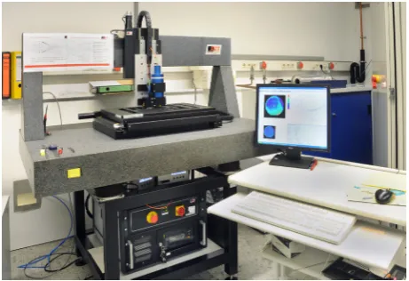
The MicroProf® system, as shown in Fig. 1, consists of a
tabletop and a yoke made of massive granite, which is mounted on a pneumatic-mechanical system ensuring a decoupling of mechanical disturbance from the floor. On the granite tabletop, a XY-stage is attached with a travel of 420 mm and 310 mm, respectively, thus defining the maximum dimensions of a sample that can be scanned during a measurement. Different fixtures can be mounted on the table, appropriate for holding the particular sample and the calibration measures needed for the determination of the total thickness variation (TTV) of a sample.
Fig. 1. MicroProf®-system.
The sensor head is situated on a vertical slide with a travel of 160 mm thus defining the maximum height of samples to be measured.
On the sensor head, multiple devices can be mounted in parallel in order to measure the same place on a sample with different methods, the lateral offset of the devices being automatically corrected via the controlling software. In our current setup, a CCD camera for sample positioning and two chromatic point sensors are mounted on the sensor head.
We have one sensor with a measuring range for 25 mm and a working distance of 80 mm, which allows for measuring large steps and very wavy samples with a lateral resolution of 14 µm and a vertical resolution of 8 µm.
Furthermore, two sensors with a measuring range of 600 µm and a working distance of 6.5 mm are available. They have a lateral resolution of 1 – 2 µm and a vertical resolution of 200 nm. They are mounted vertically aligned in a so-called TTV arrangement, the second sensor being fixed upside down to the granite table plate thus “looking” to the sample from the bottom side. For a TTV measurement, the system has to be calibrated at first with a standard measure that has a thickness in the range of ± 0.6 mm to that of the sample. After the calibration the thickness variation and the topology of
the top and bottom surfaces of the sample can be measured simultaneously.
2.2 Software
The Acquire software controls the FRT metrology tools and all sensors. This software allows fast and easy manual measurements in 1D (line) or 2D (area) and gives a quick impression of the measurement data.
FRT Mark III is the analysis software for the evaluation of surface and profile measurements. It allows the easy and efficient evaluation of surface structures and parameters according to common international standards (DIN EN ISO, SEMI, etc.). Versatile 3D views represent the surface data in realistic detail.
2.3 Measuring principle
The measuring principle is depicted in Fig. 2. An optical fibre transfers white light from a halogen lamp to the small and passive sensor head. The optical system in the head contains an aspheric lens with strong chromatic aberration that spreads the different wavelengths of the white light in vertical direction so that the focus for each wavelength is situated at a different distance from the end face of the fibre. Therefore, the confocal imaging of the sample surface is fulfilled for only one wavelength that is reflected back to the optical system and is then guided via the optical fibre coupler to the spectrograph. In the spectrograph, the signal height at the peak wavelength is then evaluated and translated to a topology signal.
By moving the sample on the xy-stage relative to the stationary sensor head, the sample topology or, for TTV arrangement, the sample thickness can be recorded.
3 Examples of application
To demonstrate the versatility of the system some examples for measurements with the MicroProf® will be
shown in the following paragraphs.
3.1 Test step
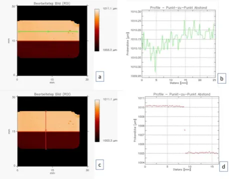
To get a first impression, two standard stainless steel measures with a thickness of 1.01mm and 1.005 mm, respectively, are placed side by side such creating a step with a height of 5 µm. In Fig. 3 the thickness data are shown in a 3-dimensional plot.
Fig. 3. 3D-plot of a 5 µm step.
In Fig. 4a and c the same measurement data as in Fig. 3 are presented in a 2-dimensional plot with the thickness now being colour-coded. The thickness values along the green line in 4a and the red line in 4c are plotted in the profile graphs in the pictures 4b and 4d on the right. The profile graph in 4b along the green line runs parallel to the plane of the 1.01 mm standard measure demonstrating the vertical accuracy of the system. The profile graph in 4d runs across the step thus showing the accuracy of mapping the sharp step.
Fig. 4. 2D colour-coded thickness data of the test step with profile lines parallel to the plane in 4a and across the step in 4c. 4b and 4d show the thickness data along the profile lines.
3.2 Monitoring preparation steps
The TTV-measurement is a mighty tool to monitor the surface structure and the sample shape after each preparation step. In Fig. 5 the thickness measurement of a carbon sample is shown as a colour-coded 2-dimensional plot after first lapping the sample (5a) and then after polishing (5c) with the corresponding graphs along the profile lines (5b and 5d respectively).
Fig. 5. Thickness of a carbon sample after lapping (top) and after polishing (bottom) 2D colour-coded (a and c) and in a graph along the profile lines (b and d).
It is clearly visible that the surface structure after lapping (Fig. 5a and 5b) is microscopically very rough, that the sample surfaces are very flat but that the whole sample is a bit wedge-shaped (Δ ~ 15 µm along the red profile line). After polishing (Fig. 5c and 5d) the surface structure is much smoother but the wedge shape remains. The sample shape is more convex and globular, the edges of the sample being thinner than the centre.
This is essential information for the application of the target since the user has to decide if the homogeneity of the sample is more important or the smoothness of the surface(s). Visualizing such effects is very instructive for the users.
3.3 Quality control for purchased targets
Some materials like e.g. beryllium cannot be produced or reshaped in-house because of safety restrictions. Especially for those samples, it is important to have a reliable characterization since the specification of the producer is often not very significant or even incorrect.
profile lines clearly show that the sample with 1 mm nominal thickness (Fig. 6 bottom row) is much more homogeneous in thickness compared to that of the 1.46 mm sample ( Fig.6 top row) which is about 5% thinner in the centre compared to the edge.
This difference in quality can also be seen in the statistical evaluation in the last column of Fig. 6, which can be performed automatically with the Mark III software.
Fig. 6. Thickness evaluation of two beryllium samples with a nominal thickness of 1.46 mm (top) and 1.0 mm (bottom). From left to right: Thickness values as photorealistic view, 2D colour-coded, as graph along the profile lines, and the statistical evaluation (with the standard deviation from the mean).
3.4 Quality control of degraders
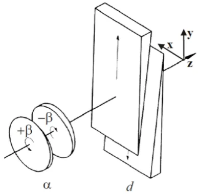
A special challenge is the measuring of large parts that are not flat but wedge-shaped like the degrader system shown schematically in Fig. 7. Since the sensors have a measuring range of only 0.6 mm, a slope of more than that cannot be measured at once.
Fig. 7. Schematic drawing of the degrader system of the Fragment Separator [3].
In the following, the measurement of one of the wedged-shaped disks with a diameter of 330 mm and a thickness of 0.5 mm to 3.2 mm from one end to the other is shown in Fig. 8 on the left. The disk is mounted on the specimen holder with the flat side down, since the bottom sensor of the setup is fixed in position, and such that the slope on the upper side of the disk is increasing from left to right. Since the disk has no stop angle, the
disk is at first placed by visual judgement and then the alignment is refined by measuring the thickness parallel to the edge where the thickness should be constant for an ideal alignment of the disk. If a variation in the thickness is measured the disk position is corrected manually, then the thickness is measured again and so on until a satisfactory alignment is obtained.
Fig. 8. A degrader disk mounted on the MicroProf®-table (left)
and the schematic drawing of the disk with the overlapping measurement areas T1 – T5.
Since the total thickness difference across the disk is 2.7 mm, the measurement is subdivided into 5 overlapping parts, as indicated in Fig. 8 on the right. For each measurement part, the upper sensor has to be shifted upwards and a new calibration with an adequate standard measure has to be conducted.
The data obtained are then exported in ASCII-format and can be further evaluated with standard codes. Fig. 9 shows the colour-coded data of the 5 partial measurements, assembled and fitted for an overview of the quality of the whole part. As a result, the accuracy of the part was sufficient for the operation in the degrader system.
Fig. 9. Assembled and fitted data of thickness [4] of the degrader disk coming from the overlapping measurement areas measurements T1 – T5 as shown in Fig.8.
4
Summary and perspectives
The described applications showed some of the powerful features of the Microprof®-system we already
In the future, we want to explore the system further to expand the measuring and evaluation possibilities. As a long-term perspective, we could consider extending our system with an additional sensor like for example an Atomic Force Microscope or a Film Thickness sensor.
References
1. B. Kindler, H. Brand, W. Hartmann, J. Steiner, J. Klemm and B. Lommel; Nucl. Instr. and Meth. A 480,160-165 (2002)
2. https://frtmetrology.com/en/
3. H. Geissel et al., Nucl. Instrum. Meth. B 70, 286 (1992)