Available Online atwww.ijcsmc.com
International Journal of Computer Science and Mobile Computing
A Monthly Journal of Computer Science and Information Technology
ISSN 2320–088X
IJCSMC, Vol. 4, Issue. 5, May 2015, pg.278 – 286
RESEARCH ARTICLE
Evaluation of Machine Learning
Algorithms in Artificial Intelligence
Ali Heydarzadegan1, Yaser Nemati2, Mohsen Moradi3
1,2 Department of Computer Engineering, Beyza Branch, Islamic Azad University, Beyza, Iran 3
Department of Computer Engineering, Firoozabad Branch, Islamic Azad University, Firoozabad, Iran
1 [email protected]; 2 [email protected]; 3 [email protected]
Abstract—Machine learning is a branch of artificial intelligence science i.e. the systems that can learn data. For example, a machine learning system can learn e-mail receiving and distinguish the difference between spam and non-spam message from each other. After training, the system can put new messages in their folders using classification. Currently, we do not know how to program computers in order to human learn more efficient. Although the methods that have been discovered operate very effectively for certain purposes, not suitable for all purposes. For example, machine learning algorithms are commonly used in data mining. Even in areas where data are concerned, these algorithms operate and result much better than other methods. For example, in issues such as speech recognition, algorithms based on machine learning resulted much better than the other methods. Apparently, it seems that our knowledge of computers will improve gradually. Certainly, it can be said that the topic of machine learning play a highly significant role in the field of computer science and game technology. This paper describes machine learning algorithms, feature selection methods, dimensions reduction, and deleting of useless data.
Keywords— Decision Tree; The Nearest K Neighbor; Regression; Neural Network; Support Vector Machine.
I. INTRODUCTION
II. THEDECISIONTREEALGORITHM
Learning by decision-tree is one of the most versatile and efficient inductive (supervised) learning methods [10-12]. This method is used in learning of discrete and error bearing data. Therefore, learning with this method is a method of estimating the objective functions with discrete values. In tree learning, the estimated function will be determined by a decision tree. The obtained trees can also be displayed as a set of If-then orders so that its evaluation will be easier for human beings.
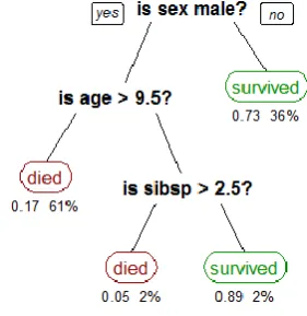
Decision tree classifies samples by sorting them from the roots to the leaves of the tree. In the tree, each node specifies the feature of the sample and each branch (which is outside the node) specifies the irrelevant amounts of the feature. First, to classify each sample we begin from the root, any feature that we achieve to we come down from a branch of the tree that matches the characteristics of the sample. This process will also continue for the sub trees to reach sample category [11-15] .The following figure is an example of this type of tree.
Fig. 1 Example of an decision tree.
Although many tree learning methods with different needs and abilities have been presented, most of the decision trees are more convenient for learning issues with following introduced features [15-19]:
• Samples are specified by sorted pairs of features and target functions. Examples of these issues are sorted by a set of constant features and their values. The most comfortable situation for decision tree is that each feature can encompass a few of the values.
• The values of target function have discrete output.
• Training data can have errors. Tree learning methods can adapt to the error in the training data, it does not matter that the value of target function is sample or one of the features is reported falsely.
Because many of practical problems have above features, the decision tree learning is very useful. As far as it can be used in issues such as medical diagnosis, detection of equipment failure, and diagnosis of loan risk based on delayed payback. Such issues that the aim of learning is classifying samples in one of the available categories are called classification [24].
III.THENEARESTKNEIGHBOR
number of samples in each class is counted and new sample is attributed to categories that the greater number of neighbors belongs to.
K is a parameter that must choose the best value by mutual validation. The nearest neighbor needs to define a distance function to find the nearest neighbor. Usual method for numerical input, their selection is carried out by the normalization of mean and division of standard deviation. Euclidean distance is used for independent input, otherwise Mehnalubis distance is used. Jaccard distance can be used for binary features [20].
The strength of K- nearest neighbor as a model does not need simple training. More data cause automatically higher learning (and old data can be deleted). Although the data need to be organized by the tree and also to find the smallest neighbor with time complexity O (LOG N) that is more than O (N), on the other hand, the weakness of k-NN is that can not well tolerated high dimensions [22,23].
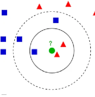
Fig. 2 Example of an KNN.
Top figure shows an example of KNN classification [24]. Test sample (green circle) should classify by first class of blue squares or second class of red triangles. If the value of K = 3, it should be allocated to the second class (circle with solid line), because there are only two triangles and a square in the inner ring, but if the value of K = 5, it is allocated to first-class, (Circle with dash line) because three squares and two triangles were located within this class.
IV.REGRESSION
Analysis of linear regression includes a response variable, Y, and a forecast variable, X. This is the simplest form of regression where Y is a linear function of X.
( 1 )
y
b Wx
Where the variance, Y, is constant and b and W are the regression coefficients for the intercept and slope, respectively [25]. Coefficients b and w can be thought as the weight and its equivalent can be written as follow:
( 2 )
0 1
y
w
w x
includes data points (x1, y1), (x2, y2), ..., (x | D |, y | D |).Regression coefficients can be estimated using the following equation.
( 3 ) 1 2 1 ( )( ) ( ) D i i i D i i
x x y y
W x x
Where ( 4 ) 0 1w
y
w x
Here
x
average x x1, 2,x3,...,xD andy
average y y1, 2,y3,...,yD and coefficients0
,
1w w
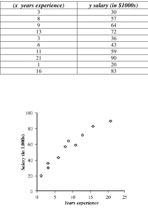
often provide a good approximation otherwise they complicate regression equation. Linear regression uses least squares methods. The following table demonstrates a set of pairs x including the number of years of experience of college graduates and Y is their salary.y salary (in $1000s) (x years experience)
30 3 57 8 64 9 72 13 36 3 43 6 59 11 90 21 20 1 83 16
Fig. 3 Example of an Regression.
between X and Y. Our model shows above relationship with y w0w x1 equation. According to above information we calculated x 9.1and y 55.4. Substitution of these values in equations (1) and (2), gives us the following values.
1 2 2 2
(3 9.1)(30 55.4) (8 9.1)(57 55.4) ... (16 9.1)(83 55.4)
(3 9.1) (8 9.1) ... (16 9.1)
w
0 55.4 (3.5)(9.1) 23.6
w
Therefore, the linear equation of least squares with high values was achieved.
23.6 3.5
Y
X
Using this equation, we can predict the relationship between salary and experience. For example, one with 10 years of experience should make salary of $ 58,600 [17].
V. SUPPORTVECTORMACHINE(SVM)
The first algorithm to classify and categorize the patterns was presented by Fisher in 1936 and its criterion for optimization was error reduction of classified training data. Many of the methods and algorithms that have been presenting up to now to design the classifications follow this strategy. In these methods, the designed classification has little generalization property. If we consider the design of classifying pattern model as an optimization problem, many of these approaches confront with the problem of local optimization in equation and caught in the trap of local optimization [25-30].
In 1965, a Russian researcher named Vladimir and Pinik took very important step in the design of classification [29,31]. He strongly established statistical learning theory and presented support vector machine according it. The support vector machines have following properties:
1. Design of classifier with a maximum extension, 2. Achieving optimal point of the total function, 3. Automatically determine the optimal topology and structure for classifier, 4. Modeling of non-linear discriminates functions using the non-linear cores and the concept of inner product in Hilbert spaces.
SVM is an algorithm that finds particular type of linear models and results in maximum margin of the page cloud. Maximizing the margin of page could result in maximum separation between classes. The nearest training points to the maximum margin of the page cloud referred to as support vectors (points). These vectors are only used to determine the boundary between the classes [18,23].
If the data are linearly and separately, SVM trains linear machine to produce an optimal level that separates data without error with the maximum distance between the screen and the closest training points. If we define the training points as [xi,yi] and the input vector as
n i
x R and the class value as yi { 1,1},i 1,.... 1 , then when the data are linearly separable, decision rules that are defined and by an optimized surface that separate binary decision classes is as the following equation.
( 5 )
1
(
(
.
)
)
n
i i i
y
sign
y a X X
b
Where Y is the equation output,
y
i is the value of training level and doter presents inner1, 2,...,
i N are support vectors. In Equation 5, the parameters of
b
anda
i determine the page cloud. If data are linearly non-separable, Equation 5 is changed to the equation below:( 6 )
1
(
(
.
)
)
n
i i i
i
y
sign
y a K X X
b
Function K X X( . i) is a Kernel function that produces domestic production to create machines with a variety of non-linear decision levels in the data space. For example, three kinds of kernel functions used in SVM are:
- Polynomial machine with kernel function of ( . ) ( . 1)d
i i
K X X X X where, d is degree of polynomial
kernel.
- Radial basis function machine with kernel function of 2 2
( . ) exp( 1/ ( ) )d
i i
K X X X X in which is
kernel bandwidth of radial basis function.
-Two layers NN machine with kernel function of K X X( . i)S X X( . i) 1/ [1 exp{ ( X X. i)c}] where c and v are Zygmoeedy S X X( . i) function so that inequality of cv is satisfied.
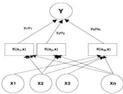
Learning process for creating decision functions is a dual structure. SVM uses optimization theory to classify that based on statistical learning theory, minimizes the error classification. Figure 4 shows the process of SVM model.
Fig. 4 Example of an SVM.
SVM has better applicable in pattern recognition, regression estimation, time-finance series forecasting, marketing, production efficiency estimation, text classification, face recognition using image, recognition of handwriting and medical diagnosis in comparison with any other learning techniques [26].
In general it can be said that SVM method in which the strength points of traditional statistical methods that are more theory-based and simple in terms of analysis, are combined. In recent years this method has been widely used in different areas of financial management such as credit rating and time series prediction [30, 31].
Method of dimensions reduction:
including topless or vector data that have n features or dimensions. This method is also called the KL method. Finding k dimension from n dimension of features can show the best form of data presentation. (where K n) The original data are predicted in a smaller space as a result it is called the dimension reduction.
Unlike the selection of features while maintaining the initial set of features that reduces the size of the feature set, PCA is a combination of essential features that substitutes a smaller set of features to reduce the dimensions. PCA often reveals relationships that have not been already experienced and this allows you to interpret the data that have not been previously interpreted.
The main method is as follows:
The characteristics of the data should be normalized, so that every feature located in its area. This stage helps to ensure that features with larger range not dominate features with smaller range.
The method calculates and presents K vector by normalized data. These vectors are perpendicular to each other and called principal components. Input data are linear combination of the principal components.
The principal components are classified in order of importance and strength or power of classification. Principal components as a new set of axes are for data with the highest variance.
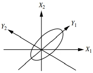
Fig. 5 Example of an PCA.
The shape of the PCA: In figure Y1 and Y2 axes are principal components for data.
Missing and waste data: Data of real world have defect, noise, and inconsistency. Therefore the methods of pre-processing and cleansing of data make effort to smooth missing values and outlier or remote points in data margins and correct data inconsistencies. Imagine that you need to analyze the data of a customer in your store. You imagine that some records have no value, such as customer income.
VI.CONCLUSION
gaps and how to use data has become an important issue. In this paper we described the machine learning algorithms, methods of feature selection, dimension reduction, and elimination of waste data. First, the duty of each method was presented, and then at the end of each algorithm, its advantages and disadvantages were expressed. The best method can be selected in different sciences according to the expression of machine learning algorithms and explaining the method, advantages, and disadvantages.
REFERENCES
[1] V. Khodadadi et al. Application Of Ants Colony System For Bankruptcy Prediction Of Companies Listed In Tehran Stock Exchange , Business Intelligence Journal, 2010.
[2] A.Aziz and A.Humayon A predicting corporate Bankruptcy:weither do we stand? Department of Economics,Loughborough University, UK,2002.
[3] Q.Yu. Machine Learning for Corporate Bankruptcy Prediction. Information and Computer Science Department, Aalto University, 2013.
[4] Y.Chiang , et al . A Hybrid Approach Of Dea, Rough Set And Support Vector Machines For Business Failure Prediction, Expert Systems With Applications, 2010.
[5] J. Bellovary et al. A review of bankruptcy prediction studies: 1930 to present. Journal of Financial Education, 33:87–114 , 2007.
[6] J. de Andrés, M. Landajo, and P. Lorca. Bankruptcy prediction models based on multinorm analysis: An alternative to accounting ratios. Knowledge-Based Systems, 30:67–77, 2012.
[7] Ming-Yuan Leon Li and Peter Miu. A hybrid bankruptcy prediction model with dynamic loadings on accounting-ratio-based and market-based information: A binary quantile regression approach. Empirical Finance, 17:818–833, 2010.
[8] W. Beaver, Financial Ratios As Predictors Of Failure, Journal Of Accounting Research 5: 71-111,1996.
[9] E. Altman,. Financial Ratios, Discriminant Analysis And The Prediction Of Corporate Bankruptcy, The Journal Of Finance 23(4): 589-609,1968.
[10] S. ho. Et al. A Hybrid Approach Based On The Combination Of Variable Selection Using Decision Trees And Case-Based Reasoning Using The Mahalanobis Distance: For Bankruptcy Prediction, Expert Systems With Applications 37 , 3482–3488,2010.
[11] T.Bell, et al. Neural Nets Versus Logistic Regression: A Comparison Of Each Model's Ability To Predict Commercial Bank Failures, Proceedings Of The 1990 D&T, University Of Kansas Symposium On Auditing Problems,1990.
[12] M. Anandarajan, And A. Anandarajan. Bankruptcy Predication Using Neural Networks, Article In Business Intelligence Techniques: A Perspective From Accounting And Finance,.Germany: Springer-Verlag,2004.
[13] J. Ohlson .Financial Ratios And The Probabilistic Prediction Of Bankruptcy, Journal Of Accounting Research 18(1): 109-131, 1980.
[14] Xu .X, Wang Y. Financial Failure Prediction Using Efficiency As A Predictor, Expert Systems With Applications, 36,366-373, 2009.
[16] T. Shumway. Forecasting bankruptcy more accurately: A simple hazard model.Journal of Business, 1:573–593, 1987.
[17] D. A. Hensher and S. Jones. Forecasting corporate bankruptcy: Optimizing the performance of the mixed logit model. Abacus, 43(3):241–364, 2007.
[18] S. Canbas, A. Cabuk, and S. B. Kilic. Prediction of commercial bank failure via multivariate statistical analysis of financial structure: The Turkish case. European Journal of Operational Research, 1:528–546, 2005.
[19] H. Frydman, E.I. Altman, and D. Kao. Introducing recursive partitioning for financial classification: The case of financial distress. Journal of Finance , 40(1):269–291, 1985.
[20] M. L. Marais, J. Patel, and M. Wolfson. The experimental design of classification models: An application of recursive partitioning and bootstrapping to commercial bank loan classifications. Journal of Accounting Research,22:87–114, 1984.
[21] H. J. Zimmermann. Fuzzy set theory and its applications. Kluwer Academic Publishers, pages 298–319, 1996.
[22] S. M. Bryant. A case-based reasoning approach to bankruptcy prediction modeling. Intelligent Systems in Accounting, Finance and Management, 6(3):195–214, 1997.
[23] C. Park and I.Han. A case-based reasoning with the feature weights derived by analytic hierarchyprocess for bankruptcy prediction. Expert Systems with Applications, 23:255–264, 2002.
[24] K. S. Shin and Y. J. Lee. A genetic algorithm application in bankruptcy prediction modeling. Expert Systems with Applications, 23:312–328, 2002.
[25] F. Varetto. A genetic algorithm application in bankruptcy prediction modeling. Journal of Banking and Finance, 22(10):1421–1439, 1998.
[26] J. H. Min and Y. C. Lee. Bankruptcy prediction using support vector machine with optimal choice of kernel function parameters. Expert Systems with Applications, 28(4):603–614, 2005.
[27] A. Cielen, L. Peeters, and K. Vanhoof. Bankruptcy prediction using a data envelopment analysis. European Journal of Operational Research, 154(2):526–532, 2004.
[28] A. I. Dimitras, R. Slowinski, R. Susmaga, and C. Zopounidis. Business failure prediction using rough sets. European Journal of Operational Research, 114(2):263–280, 1999.
[29] T. E. Mckee. Developing a bankruptcy prediction model via rough sets theory. Intelligent Systems in Accounting, Finance and Management,9(3):159–173, 2000.
[30] Ph. Simon. Too Big to Ignore: The Business Case for Big Data. Wiley. p. 89, 2013.