Multisensor Concealed Weapon Detection Using the Image Fusion Approach

University of Windsor University of Windsor

Scholarship at UWindsor

Scholarship at UWindsor

Electronic Theses and Dissertations Theses, Dissertations, and Major Papers

2016

Multisensor Concealed Weapon Detection Using the Image

Multisensor Concealed Weapon Detection Using the Image

Fusion Approach

Fusion Approach

Tuzhi Xu

University of Windsor

Follow this and additional works at: https://scholar.uwindsor.ca/etd

Recommended Citation Recommended Citation

Xu, Tuzhi, "Multisensor Concealed Weapon Detection Using the Image Fusion Approach" (2016). Electronic Theses and Dissertations. 5773.

https://scholar.uwindsor.ca/etd/5773

This online database contains the full-text of PhD dissertations and Masters’ theses of University of Windsor students from 1954 forward. These documents are made available for personal study and research purposes only, in accordance with the Canadian Copyright Act and the Creative Commons license—CC BY-NC-ND (Attribution, Non-Commercial, No Derivative Works). Under this license, works must always be attributed to the copyright holder (original author), cannot be used for any commercial purposes, and may not be altered. Any other use would require the permission of the copyright holder. Students may inquire about withdrawing their dissertation and/or thesis from this database. For additional inquiries, please contact the repository administrator via email

Multisensor Concealed Weapon Detection Using

the Image Fusion Approach

By

Tuzhi Xu

A Thesis

Submitted to the Faculty of Graduate Studies

through the Department of Electrical and Computer Engineering

in Partial Fulfillment of the Requirements for

the Degree of Master of Applied Science

at the University of Windsor

Windsor, Ontario, Canada

2016

Multisensor Concealed Weapon Detection Using the Image

Fusion Approach

by

Tuzhi Xu

APPROVED BY:

______________________________________________

S. Cheng

Civil and Environmental Engineering

______________________________________________

R. Rashidzadeh

Electrical & Computer Engineering

______________________________________________

J. Wu, Advisor

Electrical & Computer Engineering

iii

DECLARATION OF CO-AUTHORSHIP / PREVIOUS

PUBLICATION

I. Co-Authorship Declaration

I hereby declare that this thesis paper incorporates the outcome of a joint research in collaboration with, and under the supervision of, Dr. Q. M. Jonathan Wu, with the review and revision being provided by Dr. Q. M. Jonathan Wu.

I am aware of the University of Windsor Senate Policy on Authorship and I certify that I have properly acknowledged the contribution of other researchers to my thesis, and have obtained written permission from each of the co-author(s) to include the above material(s) in my thesis.

I certify that, with the above qualification, this thesis, and the research to which it refers, is the product of my own work.

II. Declaration of Previous Publication

This thesis includes one original paper that has been previously published for publication in peer reviewed journals, as follows:

Thesis Chapter

Publication title/full citation Publication status Chapter

3

T. Xu and Q. M. J. Wu, “Multisensor concealed weapon detection using the image fusion approach,” 6th International Conference on Imaging for Crime Prevention and Detection (ICDP-15), July 2015, pp. 1-7.

iv

I certify that I have obtained a written permission from the copyright owners to include the above published material in my thesis. I certify that the above material describes work completed during my registration as graduate student at the University of Windsor.

I declare that, to the best of my knowledge, my thesis does not infringe upon anyone’s copyright nor violate any proprietary rights and that any ideas, techniques, quotations, or any other material from the work of other people included in my thesis, published or otherwise, are fully acknowledged in accordance with the standard referencing practices. Furthermore, to the extent that I have included copyrighted material that surpasses the bounds of fair dealing within the meaning of the Canada Copyright Act, I certify that I have obtained a written permission from the copyright owner(s) to include such material(s) in my thesis.

v

ABSTRACT

vi

DEDICATION

vii

ACKNOWLEDGEMENTS

I would like to express my deepest gratitude to my supervisor, Dr. Jonathan Wu, for his devoted guidance, immense support and constant encouragement during my graduate study in University of Windsor. Without his excellent mentoring skills and valuable suggestion, this work would not have been done.

I would like to thank all my friends from the CVSS laboratory for their constant help. I benefited a lot from the discussion with them during my research work.

viii

TABLE OF CONTENTS

DECLARATION OF CO-AUTHORSHIP / PREVIOUS PUBLICATION ... iii

ABSTRACT ...v

DEDICATION ... vi

ACKNOWLEDGEMENTS ... vii

LIST OF TABLES ...x

LIST OF FIGURES ... xi

LIST OF ABBREVIATIONS/SYMBOLS ... xiii

CHAPTER 1 INTRODUCTION AND BACKGROUND ...1

1.1 Concealed Weapon Detection Problem...1

1.2 Introduction and Literature Review of Image Fusion ...5

1.3 Image Fusion for CWD ...12

1.3.1 Sensors Choice and Purpose of the CWD Image Fusion Algorithms ...12

1.3.2 Literature Review of CWD Image Fusion Algorithms ...13

CHAPTER 2 DOUBLE DENSITY DUAL TREE COMPLEX WAVELET TRANSFORM ...16

2.1 Discrete Wavelet Transform ...16

2.2 Double Density Discrete Wavelet Transform ...19

2.3 Dual Tree Complex Wavelet Transform ...22

2.4 Double Density Dual Tree Complex Wavelet Transform ...25

CHAPTER 3 PIXEL LEVEL IMAGE FUSION FOR CWD ...31

3.1 Procedure of the Pixel Level Image Fusion Algorithm ...31

3.2 The Low Frequency Fusion Rule ...33

3.3 The High Frequency Fusion Rule ...36

3.3.1 Noise Visibility Function...36

ix

CHAPTER 4 FEATURE LEVEL IMAGE FUSION FOR CWD ...40

4.1 Procedure of the Feature Level Image Fusion Algorithm ...40

4.2 Image Segmentation Based on GMM ...42

4.3 Feature Level Low Frequency Fusion Rule ...47

4.4 Feature Level High Frequency Fusion Rule ...49

CHAPTER 5 EXPERIMENTAL RESULTS AND ANALYSIS ...52

5.1 Quality Metrics ...52

5.2 Experiment Background ...53

5.3 Experimental Result and Analysis for Pixel Level Image Fusion ...54

5.4 Experimental Result and Analysis for Feature Level Image Fusion ...62

CHAPTER 6 CONCLUSION AND FUTURE WORK ...66

REFERENCES ...68

x

LIST OF TABLES

xi

LIST OF FIGURES

Fig. 1 Most important U.S. problems ... 1

Fig. 2 Americans’ level of concern about crime and violence ... 2

Fig. 3 Block diagram of MDB fusion algorithm... 10

Fig. 4 1D DWT analysis and synthesis filter banks ... 16

Fig. 5 1D DWT multiscale decomposition and reconstruction... 17

Fig. 6 2D DWT ... 18

Fig. 7 DDDWT analysis and Synthesis filter banks ... 20

Fig. 8 2D DDDWT filter structure ... 21

Fig. 9 The wavelet orientations of DDDWT ... 22

Fig. 10 1D DTCWT ... 22

Fig. 11 DWT filter banks for DTCWT ... 24

Fig. 12 2D DTCWT filter bank structure... 24

Fig. 13 The wavelet orientations of DTCWT ... 25

Fig. 14 Basic analysis and synthesis filter banks of DDDTCWT ... 26

Fig. 15 1D DDDTCWT filter bank structure ... 28

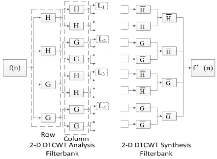
Fig. 16 2D DDDTCWT filter bank structure ... 29

Fig. 17 The wavelet orientations of DDDTCWT ... 30

Fig. 18 Block diagram of pixel level image fusion algorithm ... 32

Fig. 19 Block diagram of feature level image fusion algorithm ... 41

Fig. 20 GMM pdf of a image ... 42

Fig. 21 the block diagram of EM algorithm ... 46

Fig. 22 Four pairs of source images (a) Dataset 1 (b) Dataset 2 (c) Dataset 3 (d) Dataset 4... 54

xii

(g) DWT with proposed fusion rules (h) DTCWT with proposed fusion rules (i)

DDDWT with proposed fusion rules (j) Proposed Method ... 56

Fig. 25 Fused images of Dataset 4 (a) GP-based existing method (b) DWT-based existing method (c) DTCWT-based existing method (d) DDDWT-based existing method (e) DDDTCWT-based existing method (f) GP with proposed fusion rules (g) DWT with proposed fusion rules (h) DTCWT with proposed fusion rules (i) DDDWT with proposed fusion rules (j) Proposed Method ... 57

Fig. 26 Fused images of Dataset 3 (a) GP-based existing method (b) DWT-based existing method (c) DTCWT-based existing method (d) DDDWT-based existing method (e) DDDTCWT-based existing method (f) GP with proposed fusion rules (g) DWT with proposed fusion rules (h) DTCWT with proposed fusion rules (i) DDDWT with proposed fusion rules (j) Proposed Method ... 57

Fig. 27 Quality rating for Dataset 1 ... 60

Fig. 28 Quality rating for Dataset 2 ... 60

Fig. 29 Quality rating for Dataset 3 ... 61

Fig. 30 Quality rating for Dataset 4 ... 61

Fig. 31 Multiscale segmentation results for (a)IR/MMW (b)visual ... 62

xiii

LIST OF ABBREVIATIONS/SYMBOLS

ABBREVIATIONS DESCRIPTION

CWD Concealed Weapon Detection

HIS Intensity-Hue-Saturation

ICA Independent Component Analysis PCA Principal Component Analysis LCLS Linearly Constrained Least-Squares DWFT Discrete Wavelet frame Transform

SVM Support Vector Machines

DWT Discrete Wavelet Transform

HVS Human Visual System

NMDB non-multiscale-decomposition-based MDB multiscale-decomposition-based

AWA adaptive weight averaging

MRF Markov Random Field

NSCT non-subsampled Contourlet transform

IR Infrared

MMW millimeter wave

LPT Laplacian pyramid transform

EM expectation-maximization

DDDWT Double Density Discrete Wavelet Transform DTCWT Dual Tree Complex Wavelet Transform

DDDTCWT Double-density Dual-tree Complex Wavelet transform

1D 1-dimensional

2D 2-dimensional

pdf probability density function

GMM Gaussian mixture model

DOG Difference-of-Gaussian

SD Standard Deviation

1

CHAPTER 1

INTRODUCTION AND BACKGROUND

1.1

Concealed Weapon Detection Problem

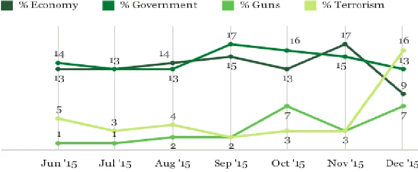
Detection of concealed weapons has been an increasingly important problem for both military and police since global terrorism and crime have grown as threats over the years. The public's concern about the threats of terrorism and crime using weapons has been rising during the past years. Terrorism has become one of the most important concerns for the public worldwide, especially after the deadly terrorist attacks in Paris and San Bernardino, California which caused hundreds of casualties. The Gallup poll released on Dec. 14, 2015 shows that 16% of Americans identified terrorism as the top challenge facing the country which is the highest percentage in a decade, shown in Fig. 1[1]. According to the Country Reports on Terrorism 2014 provided by the National

2

Consortium for the Study of Terrorism and Responses to Terrorism [2], the number of terrorist attacks worldwide in 2014 is 13,463, an increase of 35 percentage points since 2013, and the terrorist attacks resulted in more than 67,400 casualties. Another survey released on Apr. 6, 2016 by Gallup indicates that 53% of American adults claimed they worried "a great deal" about crime and violence, hitting the highest point in 15 years, shown in Fig. 2[3]. Nowadays, terrorists and criminals using firearms and explosives have become constant and increasing threats in public areas and are even more harmful comparing with the criminals with white arms like knife. The improving power and the smaller size of weapons bring more challenges to the improvement of the security of the general public as well as the safety of public assets. Therefore, the detection of weapons concealed underneath a person's clothing is one of the greatest and most urgent challenges facing the law enforcement community, crime prevention and anti-terrorism.

Easily found in airports and security-sensitive areas, security check points are established to detect concealed weapons like knives, guns and explosives. Traditional devices such as x-ray scanners, hand wands, hand-held metal detector and walk-through metal detectors are commonly used in conjunction with manual screening procedures for the searching of

3

hidden weapons. The traditional security check procedures have significant limitations despite generally providing great accuracy rate. The disadvantages of the traditional security check procedures involve:

1) Space consuming: devices like x-ray scanners and walk-through metal detectors request huge space for installation, causing reduced feasibility. 2) Time consuming: once a person could be inspected and the manual methods

slow the procedures.

3) Labor consuming: huge manpower is needed for the security check.

4) Lack of concealment: the check points are so obvious that the criminals have opportunities to make decision and take action after they discover the existence of the check points.

5) Distance requirement: the effective distances of the traditional devices are limited which could lead to insufficient reaction time for security personnel to safely deal with emergency condition.

Unsafe situation could occur due to the disadvantages. The flow of pedestrian traffic might be impeded in crowded venue like an airport terminal. The crowd trapped in a relatively small area could be a prime target for attack. Also, the safety of security staff is threatened as a result of the insufficient distance. The aforementioned 5 limitations make the traditional methods of Concealed Weapon Detection (CWD) defective and become the motivation of new solutions for CWD problem. A desirable solution should satisfy the following requirements:

4

2) The impacts on pedestrian traffic flow are limited.

3) The CWD procedures are able to take place from a standoff distance.

4) The required space of device installation is small enough to broaden the scope of applications.

5) It is ideally to provide the alarm of suspects carrying weapons without their awareness so the law enforcement is able to take action effectively and safely. 6) The less manpower requirement is preferable.

Thus, image processing methods are considered as efficient and convenient solutions for the CWD problem. Since it is difficult to provide sufficient information with a single sensor in CWD, image fusion has been identified as a key technology to improve CWD algorithms. The image fusion methods for CWD have several merits:

1) The hidden weapons can be clearly detected and recognized with the help of a small amount of personnel.

2) Several targets are able to be inspected simultaneous and the process is automatically carried out by computer program so it is possible to finish the detection procedure rapidly without stopping the pedestrians.

3) The image sensors used enable the detection from a standoff distance and are small enough to be applied in different environment.

5

1.2

Introduction and Literature Review of Image Fusion

Image fusion is the process of combining images acquired using multiple sensors to construct a new image, providing contextual enhancement of the scene being observed. Different fusion algorithms have been proposed for improving spatial and spectral resolutions of the fused images over the decades such as Brovey transform method, Intensity-Hue-Saturation (IHS) method, statistical method, Independent Component Analysis (ICA) method, numerical method and Principal Component Analysis (PCA) method. The algorithms based on a Brovey transform preserve the relative spectral contributions of each pixel but enhance the intensity or brightness component of the image. Each component of the multispectral image bands normalized using a formula is multiplied by a high-resolution co-registered data. The methods based on IHS transformation merge images by preserving most of the spectral information from the H and S components but substituting the intensity image I with histogram-matched high-resolution image. The PCA/ICA method transforms the original images into uncorrelated images and then combines the images by choosing the maximum value among all. PCA is frequently used for fusion as a statistical technique to compact the multivariate data set of inter-correlated variables redundant data into fewer uncorrelated bands.

6

At signal level, image fusion refers to the acquirement of a combined signal of the same type but with greater quality from a group of original sensor signals. Since conclusions are drawn directly from the data and independent of the choice of feature extraction algorithms, Kundur et al. [5] based their blind image restoration and classification techniques on the fusion of individual restorations resulting from single frame algorithms. Xia et al. [6] developed their signal level neural data fusion algorithms based on the Linearly Constrained Least-Squares (LCLS) statistical method.

7

measurement, based on HVS characteristic, of small arbitrary regions of wavelet transform coefficients. This method is designed for remote sensing images.

8

The symbol level is the highest abstraction level and features are classified as specific type of symbol. The sets of symbols are then fused to create the fused image. The symbol level image fusion requires classification of feature to make complex decisions and is usually costly. Zhao et al. [14] have proposed a symbol level image fusion approach based on SVM and consensus theory. The classification scheme based on SVM is used to classify the source data and the classification results are fused with consensus theory based fusion rules to obtain the fused image.

Image fusion techniques can also be classified into two group, non-multiscale-decomposition-based (NMDB) fusion methods and multiscale-non-multiscale-decomposition-based (MDB) fusion methods [15].

9

Squares technique is used to calculate the fused image. Yang et al. [18] have developed a feature level image fusion algorithm based on estimation theory. The source images are classified into regions by a graph-based image segmentation method and the regions are then analyzed to form a joint region map for the fused image. The region- level expectation-maximization (EM) fusion algorithm is developed to work on the regions modeled using Gaussian mixture distortion to estimate the model parameter and to produce the fused image. Approximate maximum likelihood estimates are produced as the EM algorithm is adopted.

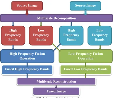
In recent years, multiscale analysis has become one of the most promising methods for image processing and a variety of MDB fusion methods, including pyramid-based methods, DWT-based methods and discrete DWFT-based methods, have been proposed. A MDB fusion method can be generally divided into three steps as shown in Fig. 3.

1) The source images are decomposed into several scale levels using multiscale transform techniques. Low frequency bands containing the approximation coefficients and high frequency bands that consist of detail coefficients are obtained.

2) Different fusion operations are applied to the low/high frequency components to fuse the transform coefficients at each level of the source image.

10

The MDB fusion approaches are able to provide both spatial and frequency domain localization. More intelligent fusion operation can be developed according to the characteristics of the multiscale decomposition representations of the images to achieve much better performance. Burt [19] proposed a multiscale gradient pyramid transform basis which filters and downsamples the input image to produce a sequence of pyramid images representing the input image information at different levels of resolution with the gradient filter for image fusion. Li et al. [20] have suggested a pixel level MDB fusion approach in which the input images are decomposed using DWT. The consistency verification is done along with the activity measurement calculated in a local computing window and maximum selection is adopted as fusion rule. Aiazzi et al. [21] have presented a fusion scheme based on generalized Laplacian pyramid. The method

High Frequency Bands Low Frequency Bands High Frequency Bands Low Frequency Bands Multiscale Decomposition

Source Image Source Image

Fused Image

Multiscale Reconstruction High Frequency Fusion

Operation

Fused High Frequency Bands

Low Frequency Fusion Operation

Fused Low Frequency Bands

11

12

1.3

Image Fusion for CWD

1.3.1 Sensors Choice and Purpose of the CWD Image Fusion Algorithms

13

temperature of their own, or reflect other temperatures in the environment, giving rise to contrast in the scene. Compared with IR camera, the most attractive feature of a MMW sensor is that the radiation wavelength of MMW is at W-Band and enables the MMW to penetrate obstacles. However, very sensitive receivers are required to amplify the signal before detection and processing into an image as the total power levels at W-Band are so low.

The purpose of image fusion algorithm for CWD application is to produce a resultant image which allows the viewer to observe:

1) The hidden weapon information from the IR/MMW image. Thus, the interested information from the IR/MMW image is the brighter (white) weapon pixels/regions surrounded by dimmer (black) the human pixels/regions.

2) The appearance information from the visual image. Thus, the target information of visual image is the appearance information of the suspects.

1.3.2 Literature Review of CWD Image Fusion Algorithms

14

15

16

CHAPTER 2

DOUBLE DENSITY DUAL TREE COMPLEX WAVELET

TRANSFORM

2.1 Discrete Wavelet Transform

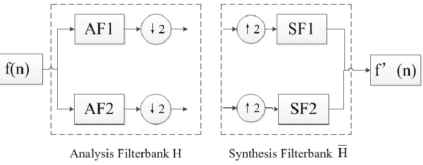
The DWT is a multiscale transform which has the ability to decompose the input signal into a multiresolution representation using a set of analyzing functions which are dilations and translations of a few wavelet functions and perfectly reconstruct the input signal. The forward and inverse 1-dimensional (1D) DWT are implemented using two-channel analysis filter bank and synthesis filter bank respectively, as shown in Fig. 4. The

DWT employs one scaling function 𝜙(𝑡), and one wavelet 𝜓(𝑡). The AF1 in Fig.4 denotes the low-pass filter associated with the scaling function and the AF2 is the high-pass filter associated with the wavelet function. AF1 is the quadrature mirror filter of AF2 of which the high-pass amplitude response is a mirror image of the low-pass amplitude response with respect to the middle frequency. Decomposition and

17

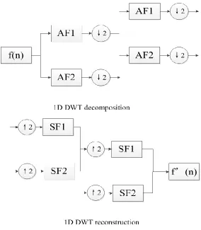
reconstruction based on the wavelet transform consists of recursively applying the 2-channel analysis filter bank on the low-pass output and performing the 2-2-channel synthesis filter bank on the reconstructed low-pass input and the original high-pass output at the same scale level, shown in Fig. 5.

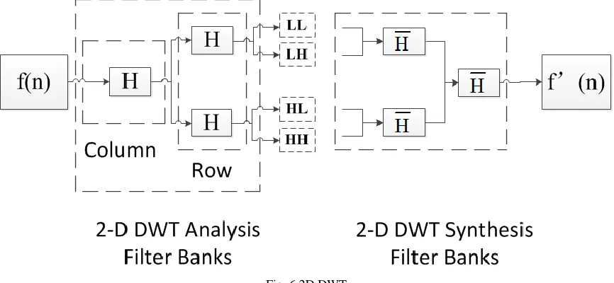
For the applications of image processing, 2-dimensional (2D) DWT is required. The filtering of 2D DWT decomposition is done first by convolving the input image with the digital analysis filter bank in the vertical direction and then downsampling the output along the column. The two output images are further processed along the row followed by down-sampling. The source image is decomposed into four subbands, LL, LH, HL and HH, as shown in Fig.6. The coefficients in LL band which is the low-pass band

18

contain the approximation information and the coefficients in the other three high

frequency subbands contain the detail information on different direction. Then the same process can be repeatedly applied to the column and row of the low-pass output bands to produce the multiscale representation of the source image. The 2D DWT is widely used in the image processing applications such as image fusion, noise attenuation, image enhancement and motion detection. The wavelet transform comes in different forms. The critically-sampled form of the wavelet transform provides the most compact representation. However, it has four main limitations:

1) Oscillations: the wavelet coefficients tend to oscillate positive and negative around singularities making singularity extraction and signal modeling challenging as the wavelets are band-pass functions.

2) Shift variance: the coefficient oscillation pattern around singularities is disturbed remarkable by a small shift of the input signal.

3) Aliasing: the repeatedly filtering of the signal with non-ideal low-pass and high-pass filters and the down-sampling operations result in substantial

19

aliasing which lead to artifacts in the reconstruction. The inverse DWT can only cancel the aliasing when there is no change on the coefficients which is unrealistic for processing.

4) Lack of directionality: the standard tensor product construction of wavelets produces a checkerboard pattern that is simultaneously oriented along several directions. DWT lack the capability of distinguishing orientations in multiple dimensions which is significant in image processing.

2.2 Double Density Discrete Wavelet Transform

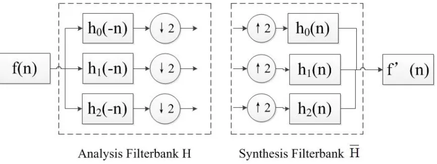
Motivated by the recognition of the limitations of DWT, DDDWT [34] have been proposed both of which are able to provide the merits such as nearly shift-invariance. The DDDWT is based on a single scaling functions 𝜙(𝑡), and two distinct wavelets 𝜓𝑖(𝑡)𝑖 = 1,2 where the two wavelets are designed to be offset from one another by one half. Assuming the low-pass and high-pass filters associated with 𝜙(𝑡), 𝜓₁(𝑡) and 𝜓₂(𝑡) are

h₀(n), h₁(n) and h₂(n) respectively. The definition of scaling and wavelet functions is given by:

𝜙(𝑡) = √2 ∑ ℎ𝑛 0(𝑛)𝜙(2𝑡 − 𝑛) (2.1)

𝜓_𝑖(𝑡) = √2 ∑ ℎ𝑛 𝑖(𝑛)𝜙(2𝑡 − 𝑛), 𝑖 = 1,2 (2.2)

20

h0(−n) associate with the scaling function and the two distinct high-pass filter are

denoted by h₁(−n) and h₂(−n). The input signal is decomposed into three subbands which are then down-sampled by 2. The lowpass subband contains the coarser

approximation information while the high-pass subbands keep the detail information of the input signal.

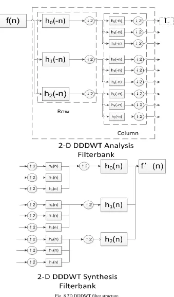
To use the DDDWT for image processing, the 2D DDDWT can be implemented simply by alternatively applying the 1D DDDWT filter bank structure first to the rows, then to the columns of an image, as shown in Fig. 8. This gives rise to nine subbands, one of which is the low-pass subbands, and the other eight of which make up the eight detail subbands. Afterwards, the same process can be repeated on the lowpass subbands to form the DDDWT multiscale decomposition.

Although the DDDWT exploits more wavelets and has the advantages as nearly shift-invariance and better wavelet smoothness, improvement is required as it lack the ability

21

of isolating the two diagonal orientations. Indicated in Fig. 9, the eight detail subbands

correspond to eight wavelet components of which two are oriented in the vertical

22

direction while another two are oriented in the horizontal direction. The rest of the wavelets do not have specific orientations, but rather combine the two diagonal

orientations, which lead to the checkerboard affect.

2.3 Dual Tree Complex Wavelet Transform

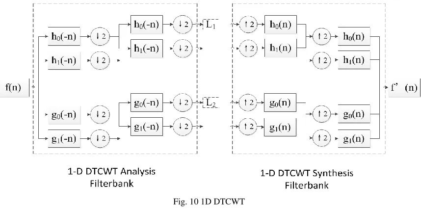
The 1D DTCWT [35] is an expansive wavelet transform and implemented using two critically-sampled DWTs in parallel on the input signal, as shown in Fig. 10. The

DTCWT has two scaling functions 𝜙ℎ(𝑡) and 𝜙𝑔(𝑡), and two distinct wavelets 𝜓ℎ(𝑡)

and 𝜓_𝑔(𝑡), forming two critically-sampled DWTs. Designed according to specific

Fig. 10 1D DTCWT

23

standards, the filters of the upper DWT are acting as the real part of a complex wavelet transform while the lower DWT filter can be interpreted as the imaginary part. Equivalently, for specially designed sets of filters, the wavelet associated with the upper DWT can be an approximate Hilbert transform of the wavelet associated with the lower DWT. If the low-pass and high-pass filters associated with 𝜙ℎ(𝑡), 𝜙𝑔(𝑡), 𝜓ℎ(𝑡) and 𝜓𝑔(𝑡) are h0(n), g0(n), h1(n) and g1(n) respectively. The scaling and wavelet functions

are defined as:

𝜙_ℎ(𝑡) = √2 ∑ ℎ_{𝑛 0}(𝑛)𝜙_ℎ(𝑡) (2.3)

𝜙_𝑔(𝑡) = √2 ∑ 𝑔𝑛 0(𝑛)𝜙𝑔(𝑡) (2.4)

𝜓_ℎ(𝑡) = √2 ∑ ℎ_{𝑛 1}(𝑛)𝜙_ℎ(𝑡) (2.5)

𝜓_𝑔(𝑡) = √2 ∑ 𝑔_{𝑛 1}(𝑛)𝜙_𝑔(𝑡) (2.6)

𝜓_𝑔(𝑡) ≈ ℋ{𝜓ℎ(𝑡)} (2.7)

where ℋ denotes the Hilbert transform.

24

information. The 12 high frequency bands associate with 12 wavelets which are oriented

25

in six directions. Every two wavelets are oriented in the same direction and one of the two wavelets performs as the real part of a complex value 2D wavelet while the other wavelet can be deem as the imaginary part of the complex-valued 2D wavelet, shown in Fig. 13.

The 2D DTCWT is nearly shift-invariant and do not have an oscillatory behavior. Moreover, all of the wavelets associated with it are oriented which is desirable for image processing.

2.4 Double Density Dual Tree Complex Wavelet Transform

The DDDTCWT [36] has been developed as complex wavelets transform combining the DTCWT and the DDDWT and possessing their merits and characteristics. The implementation of DDDTCWT is based on two pairs of analysis and synthesis filter banks which form two DDDWT structure respectively, as shown in Fig. 14. The DDDTCWT employs two scaling functions 𝜙ℎ(𝑡) and 𝜙𝑔(𝑡), and two pairs of distinct

wavelets: 𝜓_ℎ,𝑖(𝑡) , 𝜓_𝑔,𝑖(𝑡), 𝑖 = 1,2. Let h_i(n) and g_i(n) denote the four high-pass wavelet filters associated with the wavelets, 𝜓ℎ,𝑖(𝑡) , 𝜓𝑔,𝑖(𝑡), 𝑖 = 1,2. The two low-pass

26

scaling filters associated with the scaling functions, 𝜙_ℎ(𝑡) and 𝜙_𝑔(𝑡), are denoted as

h₀(n) and g₀(n).

To keep both of the properties of the DDDWT and the DTCWT, the two wavelets from the same DDDWT are designed to be offset from one another by one half, as are the filters designed for DDDWT:

𝜓_ℎ,1(𝑡) ≈ 𝜓ℎ,2(𝑡 − 0.5) (2.8)

𝜓_𝑔,1(𝑡) ≈ 𝜓_𝑔,2(𝑡 − 0.5) (2.9)

27

The two corresponding wavelets from different DDDWTs form approximate Hilbert transform pairs, as do the filters required for DTCWT:

𝜓_𝑔,1(𝑡) ≈ ℋ{𝜓ℎ,1(𝑡)} (2.10)

𝜓_𝑔,2(𝑡) ≈ ℋ{𝜓_ℎ,2(𝑡)} (2.11)

The design of the filters of DDDTCWT implementation enables the complex and directional wavelet transforms. The scaling functions and wavelets are defined through the dilation and wavelet equations:

𝜙_ℎ(𝑡) = √2 ∑ ℎ𝑛 0(𝑛)𝜙ℎ(2𝑡 − 𝑛) (2.12)

𝜙_𝑔(𝑡) = √2 ∑ 𝑔_{𝑛 0}(𝑛)𝜙_𝑔(2𝑡 − 𝑛) (2.13)

𝜓_ℎ,𝑖(𝑡) = √2 ∑ ℎ𝑛 𝑖(𝑛)𝜙ℎ(2𝑡 − 𝑛), 𝑖 = 1,2 (2.14)

𝜓𝑔,𝑖(𝑡) = √2 ∑ 𝑔𝑛 𝑖(𝑛)𝜙𝑔(2𝑡 − 𝑛), 𝑖 = 1,2 (2.15)

28

The 2D DDDTCWT is implemented by employing four oversampled 2D DDDWT in parallel to the same input image. The 2D DDDTCWT analysis and synthesis filter bank structure is shown in Fig. 16.

The implementation of the four oversampled 2D DDDWTs is realized using the combinations of the basic filter banks shown in Fig. 14. The filter banks are applied to the rows and columns of the image data alternately in the DDDWTs. Indicated in Fig. 14, the two oversampled analysis filter banks, denoted by H and G, and the two synthesis filter banks, denoted by H and G, are constructed and the synthesis filters are the time-reversed versions of the analysis filters. The 2D DDDTCWT gives rise to 36 frequency bands in

29

each level. 4 of the frequency bands are the low frequency bands containing approximation information and rest make up the 32 high frequency bands with oriented edge and texture information. The 32 wavelets associated with the 32 high frequency bands are oriented in 16 distinct directions and there are 2 wavelets oriented in each direction, as shown in Fig. 17. For each direction, one wavelet acts as the real part of a complex-valued 2D wavelet function, while the other can be interpreted as the imaginary

30

part. Therefore, the DDDTCWT possesses better directional selectivity than both the DDDWT and the DTCWT.

31

CHAPTER 3

PIXEL LEVEL IMAGE FUSION FOR CWD

3.1 Procedure of the Pixel Level Image Fusion Algorithm

The pixel level image fusion methods are popular since the cost of the schemes is commonly low and the algorithms are easy to implement. One pixel level image fusion algorithm has been developed for the application of CWD. The block diagram of the algorithm is illustrated in Fig. 18.

The algorithm is implemented in 3 steps:

1) The source images from the visual sensor and IR/WWM sensor are decomposed using the DDDTCWT. The multiscale representation of the source images in the form of low frequency bands and high frequency bands are obtained.

32

3) The fused image is created through the inverse DDDTCWT using the fused low and high frequency bands.

Experiments and comparisons demonstrate the robustness and efficiency of the proposed approach and indicate that the fusion rules can be applied to different multiscale

Fused Image Inverse DDDTCWT High Frequency Fusion

Fused High Frequency Bands

Low Frequency Fusion

Fused Low Frequency Bands High

Frequency Bands

Low Frequency

Bands

High Frequency

Bands

Low Frequency

Bands DDDTCWT

Visual Image

DDDTCWT IR/MMW Image

33

transformations. Also, it shows that the fusion result using the proposed fusion rules on DDDTCWT is superior to other combinations as well as previously proposed approaches in literature.

3.2 The Low Frequency Fusion Rule

The low frequency bands of the DDDTCWT of an image reflect the coarser approximation of the original image. The low frequency bands are similar to a compressed version of the source image with blurred texture and edge. Averaging is a convenient method to fuse the approximation coefficients of the low frequency bands and maintain the reasonable mean intensity for the fused image. However, averaging results in missing important information and reduced contrast. Thus, a low frequency fusion rule is developed based on the local contrast of the corresponding low frequency coefficients.

34

subbands, the interested coefficients containing the appearance information of the suspects are stored in the area of which the corresponding IR/MMW regions consist of the lower value (darker) coefficients indicating human body. Therefore, the preferable regions are those with larger brightness difference.

For the multiscale DDDTCWT representation of an image, only the four low frequency bands at the highest decomposition level 𝒍 are taken into consideration as the low frequency bands at other levels are produced using the four bands in the inverse DDDTCWT. The corresponding low frequency bands of the visual image and IR/WWM image are denoted by 𝑓_1,𝐿𝑙 _𝑖 and 𝑓_2,𝐿𝑙 _𝑖, for 𝑖 = 1,2,3,4 representing the four low frequency bands. To preserve the pertinent regions of the IR/WWM subbands, the normalized approximation coefficients 𝑓_1,𝐿

𝑖

𝑙,𝑁

and 𝑓_2,𝐿

𝑖

𝑙,𝑁

are used for measurement calculation:

𝑓_𝑘,𝐿

𝑖

𝑙,𝑁_{(𝑚, 𝑛) =} 𝑓𝑘,𝐿𝑖𝑙 (𝑚,𝑛)−𝑚𝑖𝑛(𝑓𝑘,𝐿𝑖𝑙 )

𝑚𝑎𝑥(𝑓_{𝑘,𝐿𝑖}𝑙 )−𝑚𝑖𝑛(𝑓_{𝑘,𝐿𝑖}𝑙 ), 𝑘 = 1,2 (3.1)

where (𝑚, 𝑛) is the position of the current coefficient.

The local contrast of the approximation coefficients used as the low frequency band fusion measurement is calculated as:

𝐶_𝑖(𝑚, 𝑛) =𝑆1,𝑖(𝑚,𝑛)−𝑆2,𝑖(𝑚,𝑛)

𝑆1,𝑖(𝑚,𝑛)+𝑆2,𝑖(𝑚,𝑛) (3.2)

35

𝑆_𝑘,𝑖(𝑚, 𝑛) = ∑ ∑ 𝑓_𝑘,𝐿

𝑖

𝑙,𝑁_{(𝑚 + 𝑎, 𝑛 + 𝑏)} 𝑏∈𝑆𝑝

𝑎∈𝑆𝑝 (3.3)

The size of the local calculation window is 𝑆_𝑝× 𝑆_𝑝.

The fusion rule of the low frequency band is a feature selection scheme, based on the local contrast measure 𝐶𝑖(𝑚, 𝑛), which has two modes. When the contrast of the two

corresponding coefficients is larger than a threshold 𝑇, a maximum chosen scheme is adopted and the coefficient with larger value is selected. In this case, the selected coefficient is high possible to contain the preferable information. If the contrast of the two corresponding coefficients is smaller than the threshold 𝑇, an averaging scheme combining the value of the coefficients is used to maintain the reasonable mean intensity for the fused image.

The fusion rule of the low frequency band is defined as:

𝑓_𝑓,𝐿𝑙 _𝑖(𝑚, 𝑛) = 𝑘₁𝑖 _{× 𝑓} 1,𝐿𝑖

𝑙 _{(𝑚, 𝑛) + 𝑘}

2𝑖 × 𝑓2,𝐿𝑖

𝑙 _{(𝑚, 𝑛) (3.4)}

Where 𝑘₁𝑖 and 𝑘₂𝑖 are the weights following the rule:

𝑘₁𝑖 + 𝑘₂𝑖 = 1 (3.5)

𝑘₁𝑖 is defined as:

𝑘₁𝑖 = {

1 𝑖𝑓 𝐶_𝑖(𝑚, 𝑛) ≥ 𝑇 0 𝑖𝑓 𝐶𝑖(𝑚, 𝑛) ≤ −𝑇 0.5 𝑖𝑓 − 𝑇 < 𝐶_𝑖(𝑚, 𝑛) < 𝑇

(3.6)

36

3.3 The High Frequency Fusion Rule

3.3.1 Noise Visibility Function

HVS research provides mathematical models regarding how human eyes respond to the visual stimulus of the world. Lots of research works on HVS have been proposed and applied in image processing applications as the HVS is an excellent image processor capable of detecting and recognizing image information. HVS-based model [37] was first introduced in image compression algorithms. Nowadays, different HVS models have been widely adopted in various research areas such as image enhancement, digital watermarking, image segmentation, motion estimation and image fusion. Noise Visibility Function (NVF), based on the noise visibility of an image, is one of the popular models and modelled by Voloshynovskiy [38]. NVF characterizes the local properties and indicates edge, texture and flat regions. Modelling the original image as a random variable with stationary generalized Gassain probability density function (pdf), the NVF at each pixel position can be calculated as:

𝑁𝑉𝐹(𝑚, 𝑛) = 𝑤(𝑚,𝑛)

𝑤(𝑚,𝑛)+𝜃𝛿2 (3.7)

where (𝑚, 𝑛) indicates the pixel location and 𝛿2 _{is the global variance of the image. 𝜃 is}

a tuning parameter which must be chosen for every particular image and computed as:

𝜃 = 𝐷

𝛿2

37

where D is an experimentally determined parameter and chosen as 60. 𝛿2_𝑚𝑎𝑥 is the maximum value of the local variance 𝛿2

𝑙 calculated in an 𝐿 × 𝐿 window as: 𝛿2

𝑙(𝑚, 𝑛) = 1

(2𝐿+1)2∑ ∑ (𝑥(𝑚 + 𝑘, 𝑛 + 𝑙) − 𝑥̅(𝑚, 𝑛))

2 𝐿

𝑙=−𝐿 𝐿

𝑘=−𝐿 (3.9)

With 𝑥̅(𝑚, 𝑛) is the local mean of pixel:

𝑥̅(𝑚, 𝑛) = 1

(2𝐿+1)2∑ ∑ 𝑥(𝑚 + 𝑘, 𝑛 + 𝑙)

𝐿 𝑙=−𝐿 𝐿

𝑘=−𝐿 (3.10) 𝑤(𝑚, 𝑛) is computed as:

𝑤(𝑚, 𝑛) =_{‖𝑟(𝑚,𝑛)‖}𝛾[𝜂(𝛾)]_2−𝛾 (3.11)

where 𝛾 is the shape parameter of the Gaussian distribution and is typically in the range from 0.3 to 1 for real images. The parameter 𝛾 depends on the decomposition level and can be estimated using a maximum likelihood estimate method [39].

𝜂(𝛾) and 𝑟(𝑚, 𝑛) are calculated as:

𝑟(𝑚, 𝑛) =𝑥(𝑚,𝑛)−𝑥(𝑚,𝑛)

𝛿𝑥 (3.12)

𝜂(𝛾) = √𝛤(3 𝛾⁄ )

𝛤(1 𝛾⁄ ) (3.13) 𝛤(. ) is the standard gamma function and defined as:

𝛤(𝑡) = ∫ 𝑒∞ −𝑢_𝑢𝑡−1_𝑑𝑢

0 (3.14)

38 3.3.2 The High Frequency Fusion Rule

The DDDTCWT high frequency band coefficients of an image contain most of the edge and texture information. The higher value of a coefficient represents a more significant change of the pixel values and indicates the edge or texture information.

The purposed of the high frequency band fusion is to better preserve the edge and texture information. As NVF is a measure of the edge and texture region based on local window calculation, the local energy of the detail coefficients can act as an additional factor to further improve the performance. A high frequency fusion rule is developed base on the combination measure of NVF and local energy. The core idea is to use the local energy weighted NVF as the texture masking function to extract all texture and edges from all high-frequency bands and select most prominent texture and edges for fused images.

For the DDDTCWT of an image, 32 high frequency bands are produce at each decomposition level. The high frequency bands from all decomposition levels are fused under the same rule. Thus, given a detail subband 𝑓_1,𝐻𝜃 _𝑖 and its corresponding detail subband 𝑓_2,𝐻𝜃 _𝑖 at decomposition level 𝜃 and 𝑖 = 1,2, … ,32 indicating different subbands of the same level, the measurement of a high frequency band coefficient located in (𝑚, 𝑛) is defined as:

𝐷_𝑓

39

where 𝑁𝑉𝐹_𝑥(𝑚, 𝑛) represents the NVF value of the coefficient calculated in a 𝑆_𝑝× 𝑆_𝑝window centred at (𝑚, 𝑛) in the frequency band 𝑥 and 𝐸_𝑥(𝑚, 𝑛) is the local energy weight computed in the same window of the subband 𝑥:

𝐸_𝑥(𝑚, 𝑛) = ∑ ∑ [𝑥(𝑚 + 𝑎, 𝑛 + 𝑏)]2 𝑏∈𝑆𝑝

𝑎∈𝑆𝑝 (3.16)

The larger energy of a detail coefficient represents more detail information.

The fusion rule of the high frequency band is also a feature selection scheme, based on the local energy weighted NVF value, which has two modes. The texture and edge information from whichever image is desirable. When the measurement value of the two corresponding coefficients is different, a maximum chosen scheme is adopted and the coefficient with larger measurement value is selected. This means the coefficient with more texture and edge information is chosen. Only if the measurement value of the two corresponding coefficients is equal, an averaging scheme combining the value of the coefficients is applied. The fusion rule of detail coefficients can be interpreted as:

𝑓_𝑓,𝐻

𝑖

𝜃 _{(𝑚, 𝑛) = 𝑘}

3𝑖 × 𝑓1,𝐻𝑖

𝜃 _{(𝑚, 𝑛) + 𝑘}

4𝑖 × 𝑓2,𝐻𝑖

𝜃 _{(𝑚, 𝑛) (3.17)}

Where 𝑘₃𝑖 and 𝑘₄𝑖 are the weights following the rule:

𝑘₃𝑖 + 𝑘₄𝑖 _{= 1 (3.18)}

𝑘₃𝑖 is defined as:

𝑘₃𝑖 =

{

1 𝑖𝑓 𝐷𝑓_1,𝐻𝑖𝜃 (𝑚, 𝑛) > 𝐷𝑓_2,𝐻𝑖𝜃 (𝑚, 𝑛) 0 𝑖𝑓 𝐷_𝑓

1,𝐻𝑖𝜃 (𝑚, 𝑛) < 𝐷𝑓2,𝐻𝑖𝜃 (𝑚, 𝑛)

0.5 𝑖𝑓 𝐷_𝑓

1,𝐻𝑖𝜃 (𝑚, 𝑛) = 𝐷𝑓2,𝐻𝑖𝜃 (𝑚, 𝑛)

40

CHAPTER 4

FEATURE LEVEL IMAGE FUSION FOR CWD

4.1 Procedure of the Feature Level Image Fusion Algorithm

The feature level image fusion methods are less sensitive to noise and the utilization of the feature characteristics leads to more intelligent fusion schemes improving the performance of the algorithms. A feature level image fusion approach has been developed for the application of CWD. The block diagram of the algorithm is illustrated in Fig. 19.

The algorithm includes 4 steps:

1) The source images from the visual sensor and IR/WWM sensor are decomposed using the DDDTCWT. The low frequency bands and high frequency bands of the source images are produced.

2) Multiscale image segmentation scheme based on GMM is applied to the multiscale representation of the source images to create the label matrix for visual and IR/WWM image respectively.

41

4) The fused image is created through the inverse DDDTCWT using the fused low and high frequency bands.

High Frequency Fusion Low Frequency Fusion

Fused High Frequency Bands

Fused Image Inverse DDDTCWT

Fused Low Frequency Bands High Frequency Bands Low Frequency Bands Visual Image DDDTCWT Multiscale Segmentation Visual Label Matrix High Frequency Bands Low Frequency Bands DDDTCWT IR/MMW Image Multiscale Segmentation IR/MM W Label Matrix

42

Experiments and comparisons demonstrate the efficiency of the developed approach and indicate that the feature level image fusion owns advantages on feature preservation.

4.2 Image Segmentation Based on GMM

GMMs are flexible and powerful statistical models that assume all the data points are characterized by a mixture of a finite number of Gaussian distributions with unknown parameters. The GMM pdf is represented as a weighted sum of component Gaussian densities, as shown in Fig. 20. Each component density of GMM is a Gaussian distribution.

The GMM is a well-known probabilistic model which has been widely used in applications, such as image fusion, image sequence analysis, image compressions and image segmentation, due to its simplicity and ease of implementation. In the feature level image fusion algorithm, a GMM segmentation algorithm based on MRF [40] is used to classify the DDDTCWT coefficients into regions and produce the label matrixes. The segmentation algorithm incorporates spatial relationships among neighboring pixels in a

43

simpler metric to make the scheme fast and easy to implement. An EM algorithm is directly applied to optimize the parameters.

The main objective of the GMM based segmentation approach is to classify the image pixels into K labels. Let 𝑥_𝑖 𝑖 == (1,2, . . . , 𝑁), present an observation at the 𝑖𝑡ℎ pixel of an image with dimension 𝐷. The neighborhood of the 𝑖𝑡ℎ pixel is denoted by 𝛿𝑖. Consider

there are K random sources, labeled as Ω_𝑗, 𝑗 = (1,2, . . . , 𝐾), of which each characterized by a Gaussian pdf:

Φ(𝑥𝑖|Θ) = 1 2𝜋𝐷/2_|Σ

𝑗|

1 2⁄ 𝑒𝑥𝑝 {−

1

2(𝑥𝑖 − 𝜇𝑗) 𝑇

Σ𝑗−1(𝑥𝑖 − 𝜇𝑗)} (4.1)

where Σ_𝑗 denotes the 𝐷 × 𝐷 covariance matrix and |Σ_𝑗| is the determinant of Σ_𝑗. 𝜇_𝑗

denotes the D-dimension mean vector and Θ_𝑗 = {𝜇_𝑗, Σ_𝑗} . The density function at an observation 𝑥_𝑖 is given by:

𝑓(𝑥_𝑖|Π, Θ) = ∑𝐾_𝑗=1𝜋_𝑖𝑗Φ(𝑥_𝑖|Θ) (4.2)

where Π = 𝜋_𝑖𝑗, 𝑖 = (1,2, . . . , 𝑁), 𝑗 = (1,2, . . . , 𝐾) is the set of prior distributions modeling the probability that pixel 𝑥𝑖 belongs to the label Ω𝑗, which satisfies the constraints:

0 ≤ 𝜋_𝑖𝑗 ≤ 1 𝑎𝑛𝑑 ∑𝐾_𝑗=1𝜋_𝑖𝑗 = 1 (4.3)

44

𝑝(𝑋|Π, Θ) = ∏𝑁𝑖=1𝑓(𝑥𝑖|Π, Θ)= ∏𝑖=1𝑁 ∑𝐾𝑗=1𝜋𝑖𝑗Φ(𝑥𝑖|Θ) (4.4)

Taking the spatial correlation between the neighboring pixels into consideration, the MRF distortion is applied to reduce the sensitivity of noise and illumination. The posterior probability density function can be written as:

𝑝(Π, Θ|𝑋) ∝ 𝑝(𝑋|Π, Θ)𝑝(Π) (4.5)

where 𝑝(Π) is the MRF distortion:

𝑝(Π) = 𝑍−1𝑒𝑥𝑝 {−1

𝑇𝑈(Π)} (4.6) 𝑍 denotes a normalizing constant and 𝑇 is a temperature constant. 𝑈(Π) is the smoothing function:

𝑈(Π) = − ∑𝐾_𝑖=1∑𝐾_𝑗=1𝐺_𝑖𝑗(𝑡)log 𝜋_𝑖𝑗(𝑡+1) (4.7)

where 𝐺_𝑖𝑗(𝑡) is a factor 𝐺_𝑖𝑗 based on the posterior probability 𝑧_𝑖𝑗 and 𝜋_𝑖𝑗 at the 𝑡𝑡ℎ

iteration step and calculated as:

𝐺_𝑖𝑗(𝑡) = exp {𝛽

2𝑁𝑖∑ (𝑧𝑚𝑗

(𝑡) _{+ 𝜋} 𝑚𝑗 (𝑡)₎

𝑚∈𝛿𝑖 } (4.8)

where 𝛽 is the temperature value controlling the smoothing prior and set to 12. 𝛿_𝑖 is a square 5 × 5 window and 𝑁𝑖 denoting the number of pixel in 𝛿𝑖 is equal to 25. The

log-likelihood function can be written as:

𝐿(Π, Θ|𝑋) = log 𝑝(Π, Θ|𝑋)

= ∑𝑁𝑖=1log{∑𝐾𝑗=1𝜋𝑖𝑗(𝑡+1)Φ(𝑥𝑖|Θ(𝑡+1))}− log 𝑍 + 1

𝑇∑ ∑ 𝐺𝑖𝑗

(𝑡)

log 𝜋𝑖𝑗(𝑡+1) 𝐾

𝑗=1 𝐾

45

where 𝑍 and 𝑇 are set to 1. Maximizing the log-likelihood function will lead to an increase in the value of the objective function:

𝐽(Π, Θ|𝑋) = ∑𝑁𝑖=1∑𝐾𝑗=1𝑧_𝑖𝑗(𝑡){log 𝜋𝑖𝑗(𝑡+1)+ log Φ(𝑥𝑖|Θ(𝑡+1))} +

∑𝐾𝑖=1∑𝐾𝑗=1𝐺_𝑖𝑗(𝑡)log 𝜋𝑖𝑗(𝑡+1) (4.10)

The segmentation is then realized by applying the EM scheme to optimize the parameters in order to maximize the objective function 𝐽(Π, Θ|𝑋). When the parameter-learning phase is complete, the determination of the classification of each pixel 𝑥_𝑖 is made based on the optimized posterior probability:

𝑥_𝑖 ∈ Ω_𝑗: 𝑖𝑓 𝑧_𝑖𝑗 ≥ 𝑧_𝑖𝑘, 𝑘 = (1,2, … , 𝐾) (4.11)

Each pixel is assigned to the label with the largest posterior probability 𝑧_𝑖𝑗.

The EM algorithm procedure is summarized as follows and shown in Fig. 21:

1) Initialize the parameters{Π, Θ} using a k-mean algorithm: the prior distributions

𝜋_𝑖𝑗, the mean 𝜇_𝑗 and the covariance Σ_𝑗.

2) E step: Evaluate the value 𝑧𝑖𝑗 and update the factor 𝐺𝑖𝑗.

3) M step: update the parameters {Π, Θ}.

46

The DDDTCWT representation of an image at every scale level can be deemed as an image with 36 dimensions. Thus the GMM segmentation algorithm is applied to the subbands of the source image at each level to create the label matrixes. In order to separate the weapon coefficients from the background coefficients, then the region map of the IR/MMW subbands is relabeled to ensure that the regions are continuous.

Initialize the Parameters

𝐦𝐞𝐚𝐧 𝝁_𝒋, 𝐜𝐨𝐯𝐚𝐫𝐢𝐚𝐧𝐜𝐞 𝚺_𝒋, 𝐩𝐫𝐢𝐨𝐫 𝐝𝐢𝐬𝐭𝐫𝐢𝐛𝐮𝐭𝐢𝐨𝐧 𝛑_𝒋

M step: update

𝐦𝐞𝐚𝐧 𝝁_𝒋, 𝐜𝐨𝐯𝐚𝐫𝐢𝐚𝐧𝐜𝐞 𝚺_𝒋, 𝐩𝐫𝐢𝐨𝐫 𝐝𝐢𝐬𝐭𝐫𝐢𝐛𝐮𝐭𝐢𝐨𝐧 𝛑_𝒋

Check the convergence of the likelihood function or parameters

Yes

No

𝒙_𝒊 ∈ 𝛀_𝒋: 𝐢𝐟 𝐩𝐨𝐬𝐭𝐞𝐫𝐢𝐨𝐫 𝐩𝐫𝐨𝐛𝐚𝐛𝐢𝐥𝐢𝐭𝐲 𝒛_𝒊𝒋> 𝒛_𝒊𝒌;

True

E step: Evaluate the value 𝒛_𝒊𝒋 and update 𝑮_𝒊𝒋

47

4.3 Feature Level Low Frequency Fusion Rule

The preferable regions for the CWD application are the region containing concealed weapon information from the IR/MMW image and the areas that the personal identification information is stored from the visual image. In the feature level low frequency image fusion scheme, the region saliency of low frequency band is used as measurement.

48

Let Ω_𝑖𝑣, 𝑖 = (1,2, . . . , 𝑁) and Ω_𝑗𝑠, 𝑗 = (1,2, . . . , 𝐾) denote the segmentation labels of the highest level visual image subbands and IR/MMW image subbands, respectively. The region color mean of a low frequency band can be calculated as:

𝑠𝑐_𝑛𝑘(𝑙) = 1

𝑁𝑙∑ 𝑥𝑛

𝑘_{(𝑟, 𝑐)}

𝑥𝑛𝑘(𝑟,𝑐)∈Ω𝑙𝑘 𝑘 ∈ {𝑣, 𝑠}, 𝑙 ∈ {𝑖, 𝑗} (4.12)

where 𝑘 ∈ {𝑣, 𝑠} distinguishes the source image and 𝑙 ∈ {𝑖, 𝑗} indicates the region labels.

𝑥_𝑛𝑘_{(𝑟, 𝑐) is an approximation coefficient located at (𝑟, 𝑐) and 𝑁}

𝑙 is the total number of the

coefficients belong to the label Ω_𝑙𝑘. 𝑛 ∈ {1,2,3,4} denotes the 4 low frequency bands of a source image at the highest level. The spatial position 𝑠𝑝𝑛𝑘(𝑙) of a region labeled as Ω𝑙𝑘 is

defined as the center location of the region. One factor of the saliency measure is created based on the color contrast cue that the salient stimulus should be distinct from its neighborhood. Thus, the color contrast factor is designed to be proportional to the color contrast of the region and its neighbor regions:

𝑐𝑜𝑛𝑠_𝑛𝑘_{(𝑎)_𝑜 = 𝛼 ∑ 𝑒𝑥𝑝 {−𝑑(𝑠𝑝}

𝑛𝑘(𝑎), 𝑠𝑝𝑛𝑘(𝑏))} × 𝑑(𝑠𝑐𝑛𝑘(𝑎), 𝑠𝑐𝑛𝑘(𝑏))

𝑎≠𝑏 (4.13)

where 𝑑(𝑥, 𝑦) is the normalized Euclidean distance between 𝑥 and 𝑦.𝛼 is a weight to better preserve the weapon information and calculated as:

𝛼 = {

𝑠𝑐𝑛𝑘(𝑎)

𝜇𝑛𝑘 𝑘 = 𝑠

1 𝑘 = 𝑣

(4.14)

Where 𝜇_𝑛𝑘 _{is the intensity mean of the low frequency band. Another saliency factor is}

designed according to the color distribution cue that the salient objects are commonly centered and compact:

𝑛𝑑𝑖𝑠𝑠_𝑛𝑘_{(𝑎)_𝑜 = 𝛽 ∑ 𝑑(𝑠𝑝}

𝑛𝑘(𝑎), 𝑠𝑝𝑛𝑘(𝑏))

𝑎≠𝑏 (4.15)

49

𝛽 =𝑁𝑎

𝑁𝑛𝑘 (4.16)

𝑁𝑎 is the total coefficients of the region and 𝑁𝑛𝑘 is the number of the total coefficients of

the subband. The two factor 𝑐𝑜𝑛𝑠𝑛𝑘(𝑎)_𝑜 and 𝑛𝑑𝑖𝑠𝑠𝑛𝑘(𝑎)_𝑜 are then normalized to [0, 1],

denoted by 𝑐𝑜𝑛𝑠𝑛𝑘(𝑎) and 𝑛𝑑𝑖𝑠𝑠𝑛𝑘(𝑎). The region saliency is computed as:

𝑠𝑎𝑙𝑛𝑘(𝑎) = 𝑐𝑜𝑛𝑠𝑛𝑘(𝑎) × (1 − 𝑛𝑑𝑖𝑠𝑠𝑛𝑘(𝑎)) (4.17)

A saliency map 𝑆𝑛𝑘 can be created as the coefficients belong to the same region own the

same saliency value. Therefore, the fusion rule of the low frequency bands:

𝑓_𝑛𝑓(𝑟, 𝑐) = 𝑘₁𝑖 _{× 𝑓}

𝑛𝑠(𝑟, 𝑐) + 𝑘2𝑖 × 𝑓𝑛𝑣(𝑟, 𝑐) (4.18)

where 𝑓𝑛𝑠(𝑟, 𝑐), 𝑓𝑛𝑣(𝑟, 𝑐) denote the corresponding approximation coefficients from the

IR/MMW and visual image. 𝑘₁𝑖 and 𝑘₂𝑖 are the weights following the rule:

𝑘₁𝑖 + 𝑘₂𝑖 = 1 (4.19)

𝑘₁𝑖 is defined as:

𝑘₁𝑖 = {

1 𝑖𝑓 𝑆_𝑛𝑠(𝑟, 𝑐) − 𝑆_𝑛𝑣_{(𝑟, 𝑐) ≥ 𝑇} 0 𝑖𝑓 𝑆_𝑛𝑠(𝑟, 𝑐) − 𝑆_𝑛𝑣_{(𝑟, 𝑐) ≤ −𝑇} 0.5 𝑖𝑓 − 𝑇 < 𝑆𝑛𝑠(𝑟, 𝑐) − 𝑆𝑛𝑣(𝑟, 𝑐) < 𝑇

(4.20)

where 𝑇 is a positive threshold.

4.4 Feature Level High Frequency Fusion Rule

50

For the feature level fusion of high frequency bands, a region detail information measure scheme has been developed. The frequency tuned saliency algorithm [42] is used to generate the saliency map for the high frequency bands. A Difference-of-Gaussian (DOG) filter is applied to the high frequency bands to extract the low level features. The variance of the DOG filter is specifically designed to preserve the edge and texture information. Let Ω_𝑣,𝑚𝐿,(𝑖) 𝑖 = (1,2, … , 𝑁) and Ω_𝑠,𝑚𝐿,(𝑗) 𝑗 = (1,2, … , 𝐾) denote the labels of the visual image subbands and IR/MMW subbands, respectively. L is the decomposition level and 𝑚 = (1,2, … ,32) represents the 32 high frequency bands. A saliency map for a high frequency band 𝑓_𝑘,𝑚𝐿 at level L is obtained as:

𝑠𝑎𝑙_𝑘,𝑚𝐿 = 𝐷𝑂𝐺(𝑓_𝑘,𝑚𝐿 ) (4.21) where 𝑘 ∈ {𝑣, 𝑠} distinguishes the source images. The region saliency of a high frequency band region labeled by Ω_𝑘,𝑚𝐿,(𝑙) is given by:

𝑆𝐴𝐿𝐿_𝑘,𝑚(𝑙) = 1

𝑁_𝑘,𝑚𝐿,(𝑙)∑ 𝑠𝑎𝑙𝑘,𝑚

𝐿 _{(𝑟, 𝑐)}

𝑥_𝑘,𝑚𝐿 (𝑟,𝑐)∈Ω_𝑘,𝑚𝐿,(𝑙) (4.22)

where 𝑙 ∈ {𝑖, 𝑗} indicate the label and 𝑁_𝑘,𝑚𝐿,(𝑙) is the number of the coefficients labeled by

Ω_𝑘,𝑚𝐿,(𝑙). 𝑥_𝑘,𝑚𝐿 (𝑟, 𝑐) is a detail coefficient. The region detail information measurement is defined as:

𝑀_𝑘,𝑚𝐿 (𝑙) = 𝐸_𝑘,𝑚𝐿 _{(𝑙) × 𝑆𝐴𝐿} 𝑘,𝑚

𝐿 _{(𝑙) (4.23)}

where 𝐸_𝑘,𝑚𝐿 (𝑙) is the average energy of the subband region:

𝐸_𝑘,𝑚𝐿 (𝑙) = 1

𝑁_𝑘,𝑚𝐿,(𝑙)∑ 𝑥𝑘,𝑚

𝐿 _{(𝑟, 𝑐)}2

𝑥_𝑘,𝑚𝐿 (𝑟,𝑐)∈Ω_𝑘,𝑚𝐿,(𝑙) (4.24)

51

𝑓_𝑓,𝑚𝐿 (𝑟, 𝑐) = 𝑘₃𝑖 _{× 𝑓}

𝑠,𝑚𝐿 (𝑟, 𝑐) + 𝑘4𝑖 × 𝑓𝑣,𝑚𝐿 (𝑟, 𝑐) (4.25)

where 𝑘₃𝑖 and 𝑘₄𝑖 are the weights following the rule:

𝑘₃𝑖 + 𝑘₄𝑖 = 1 (4.26)

𝑘₃𝑖 is defined as:

𝑘₃𝑖 = 𝑀𝑃_𝑠,𝑚𝐿 (𝑟, 𝑐) (𝑀𝑃_𝑠,𝑚𝐿 _{(𝑟, 𝑐) + 𝑀𝑃}

𝑣,𝑚𝐿 (𝑟, 𝑐))

52

CHAPTER 5

EXPERIMENTAL RESULTS AND ANALYSIS

5.1 Quality Metrics

Better image fusion algorithms should preserve complimentary features from source images and should not introduce artifacts and inconsistencies. Therefore, several objective quality metrics have been used to estimate the quality of the images. Higher metrics values indicate better image quality.

1) Standard Deviation (SD): SD is able to characterize the dispersion of the pixel values of an image:

𝑆𝐷 = √∑ ∑𝑁 |𝑥(𝑖, 𝑗) − 𝑥| 𝑗=1

𝑀

𝑖=1 ⁄𝑀𝑁 (5.1)

where 𝑥(𝑖, 𝑗) is an image pixel, 𝑀 and 𝑁 are the size of the image and 𝑥 is the mean value of the image pixels.

2) Entropy: The entropy measures the information presented in an image and is defined as follows:

𝐻 = − ∑𝐿𝑖=0𝑝(𝑖)𝑙𝑜𝑔2𝑝(𝑖) (5.2)

53

3) Mutual Information (MI): MI is a measurement indicating the degree of dependence of two images. When two images are independent, the value of MI is zero.

𝑀𝐼_𝐴𝐵 = ∑ ∑ ℎ_𝐴𝐵(𝑎, 𝑏)𝑙𝑜𝑔₂ ℎ𝐴𝐵(𝑎,𝑏)

ℎ𝐴(𝑎)ℎ𝐵(𝑏)

𝐿−1 𝑏=0 𝐿−1

𝑎=0 (5.3)

where ℎ_𝐴𝐵(𝑎, 𝑏) is the normalized joint grey level histogram of images A and B. ℎ𝐴(𝑎) and ℎ𝐵(𝑏) are the normalized marginal histograms of the two

images, and 𝐿 is the number of grey levels.

MI between the fused image F and the two source images A and B is:

𝑀𝐼_𝐹𝐴𝐵 = (𝑀𝐼_𝐹𝐴 + 𝑀𝐼_𝐹𝐵)/2 (5.4) 4) Objective edge based quality 𝑄𝐴𝐵/𝐹 _{[43]: Objective edge based quality, based}

on Sobel’s operator, indicates the amount of edge information that has been transferred: 𝑄𝐴𝐵/𝐹 =∑ ∑ [𝑄 𝐴𝐹_{(𝑖,𝑗)𝑤}𝐴_{(𝑖,𝑗)+𝑄}𝐵𝐹_{(𝑖,𝑗)𝑤}𝐵_(𝑖,𝑗)] 𝑁 𝑗=1 𝑀 𝑖=1 ∑ ∑𝑁 [𝑤𝐴_{(𝑖,𝑗)+𝑤}𝐵_(𝑖,𝑗)] 𝑗=1 𝑀 𝑖=1 (5.5)

where A, B and F represent source images and the fused image, respectively.

𝑄𝐴𝐹 and 𝑄𝐵𝐹 are edge information preservation values and 𝑤𝐴 and 𝑤𝐵 are

weights.

5.2 Experiment Background

54

method [15], DTCWT-based method [31], DDDWT-based method [32] and an existing DDDTCWT-based algorithm [24], are used in the comparison.

The source images are depicted as Fig. 22.

5.3 Experimental Result and Analysis for Pixel Level Image Fusion

The performance of the proposed pixel level fusion algorithm is demonstrated through the experiments on different image datasets and the comparisons with other methods. In the experiments, the calculation window is chosen as 3 × 3 when computing the local contrast, NVF, and local energy. The highest decomposition level 𝑙 is selected as 3.

55

56

Fig. 24 Fused images of Dataset 1 (a) GP-based existing method (b) DWT-based existing method (c) DTCWT-based existing method (d) DDDWT-based existing method (e) DDDTCWT-based existing method (f) GP with proposed fusion rules (g) DWT with proposed fusion rules (h) DTCWT with proposed fusion rules (i) DDDWT with proposed fusion rules (j) Proposed Method

57

Fig. 26 Fused images of Dataset 3 (a) GP-based existing method (b) DWT-based existing method (c) DTCWT-based existing method (d) DDDWT-based existing method (e) DDDTCWT-based existing method (f) GP with proposed fusion rules (g) DWT with proposed fusion rules (h) DTCWT with proposed fusion rules (i) DDDWT with proposed fusion rules (j) Proposed Method