Gas-liquid phenomena with dynamic contact angle in cathode of proton exchange membrane fuel cells

(1)

University of Windsor University of Windsor

Scholarship at UWindsor

Electronic Theses and Dissertations Theses, Dissertations, and Major Papers

2011

Gas-liquid phenomena with dynamic contact angle in cathode of

proton exchange membrane fuel cells

Xichen Wang

University of Windsor

Follow this and additional works at: https://scholar.uwindsor.ca/etd

Recommended Citation Recommended Citation

Wang, Xichen, "Gas-liquid phenomena with dynamic contact angle in cathode of proton exchange membrane fuel cells" (2011). Electronic Theses and Dissertations. 5395.

https://scholar.uwindsor.ca/etd/5395

This online database contains the full-text of PhD dissertations and Masters’ theses of University of Windsor students from 1954 forward. These documents are made available for personal study and research purposes only, in accordance with the Canadian Copyright Act and the Creative Commons license—CC BY-NC-ND (Attribution, Non-Commercial, No Derivative Works). Under this license, works must always be attributed to the copyright holder (original author), cannot be used for any commercial purposes, and may not be altered. Any other use would require the permission of the copyright holder. Students may inquire about withdrawing their dissertation and/or thesis from this database. For additional inquiries, please contact the repository administrator via email

(2)

GAS-LIQUID PHENOMENA WITH DYNAMIC CONTACT ANGLE IN

CATHODE OF PROTON EXCHANGE MEMBRANE FUEL CELLS

by

XICHEN WANG

A Thesis

Submitted to the Faculty of Graduate Studies

through Mechanical, Automotive and Materials Engineering

in Partial Fulfillment of the Requirements for

the Degree of Master of Applied Science at the

University of Windsor

Windsor, Ontario, Canada

2011

(3)

Gas-liquid phenomena with dynamic contact angle in cathode of proton exchange

membrane fuel cells

by

Xichen Wang

APPROVED BY:

______________________________________________

Dr. Tirupati Bolisetti

Department of Civil & Environmental Engineering

______________________________________________

Dr. Ronald M Barron

Department of Mechanical, Automotive & Materials Engineering

______________________________________________

Dr. Biao Zhou, Advisor

Department of Mechanical, Automotive & Materials Engineering

______________________________________________

Dr. Amir Fartaj, Chair of Defense

Department of Mechanical, Automotive & Materials Engineering

(4)

iii

DECLARATION OF PREVIOUS PUBLICATION

This thesis includes [1] original papers that have been previously published for publication in peer

reviewed journals, as follows:

Thesis Chapter Publication title/full citation Publication status*

Chapter 5 (Partial)

X. Wang, B. Zhou, Liquid water flooding process in proton exchange membrane fuel cell cathode with straight parallel channels and porous layer, Journal of Power Sources, 196 (2011) 1776-1794.

published

I certify that I have obtained a written permission from the copyright owner(s) to include the

above published material(s) in my thesis. I certify that the above material describes work

completed during my registration as graduate student at the University of Windsor.

I declare that, to the best of my knowledge, my thesis does not infringe upon anyone’s copyright

nor violate any proprietary rights and that any ideas, techniques, quotations, or any other

material from the work of other people included in my thesis, published or otherwise, are fully

acknowledged in accordance with the standard referencing practices. Furthermore, to the extent

that I have included copyrighted material that surpasses the bounds of fair dealing within the

meaning of the Canada Copyright Act, I certify that I have obtained a written permission from the

copyright owner(s) to include such material(s) in my thesis.

I declare that this is a true copy of my thesis, including any final revisions, as approved by my

thesis committee and the Graduate Studies office, and that this thesis has not been submitted for

(5)

iv

ABSTRACT

Fundamental understanding of liquid water behaviours in the cathode of proton exchange

membrane fuel cells (PEMFC) contributes to the investigation of the liquid water management in

PEMFCs. In this work, a three-dimensional two-phase flow model using volume of fluid method

(VOF) with dynamic contact angle (DCA) is developed through user defined function (UDF) codes

and validated by comparing the simulation results with experimental results available from the

literature. An improvement is proposed and implemented for the Hoffman function to calculate

local DCAs. By employing this methodology, gas-liquid phenomena inside the cathode of PEMFCs

with porous layer and different gas flow field designs are studied and compared with the

(6)

v

DEDICATION

(7)

vi

ACKNOWLEDGEMENTS

I would like to express my feeling of gratitude to my advisor, Dr. Biao Zhou. I thank him for

providing me the opportunity to join in his laboratory and pursue my M. A. Sc. degree in

University of Windsor. His guidance, suggestions, and encouragement helped me greatly in my

research during these two years.

I would like to give sincere thanks to Dr. Tirupati Bolisetti and Dr. Ronald M Barron for serving in

my thesis committee and contributing their time and efforts. Thank Dr. Amir Fartaj for chairing

my oral defence.

I am grateful to Simo Kang, as my research partner and roommate. Also thanks to who helped

and showed their kindness to me in the MAME department and in the University of Windsor.

Finally, special thanks are given to my mother Chengfang Jing and father Jianqun Wang. Thank

you so much for supporting me and loving me heart and soul. It is my luck and honour to be your

(8)

vii

LIST OF FIGURES

Figure 1-1 Principle of a fuel cell ... 1

Figure 1-2 An exploded view of PEMFC components ... 3

Figure 1-3 Definition of dynamic contact angle ... 4

Figure 3-1 The calculated values of original and revised Hoffman function ... 13

Figure 4-1 Comparison of liquid water behaviours between numerical simulation and the experiment at t = 0.400s [33] ... 14

Figure 4-2 Numerical and experimental slug flow model conducted by Fang et al. [46] ... 16

Figure 4-3 Results comparison between Case2 (second row) and experiment (first row) ... 17

Figure 4-4 Results comparison between Case4 and experiment ... 18

Figure 4-5 (a-m) Slug flow movements with velocity field in Case2 ... 20

Figure 4-6 (a-b) Liquid distribution with DCA on the bottom wall in Case2 ... 22

Figure 4-7 Experimental setup for droplet impact model [41] ... 24

Figure 4-8(a-c) Results comparison of droplet impact model ... 25

Figure 4-9 Results comparison between SCA and DCA model of glycerine impact ... 26

Figure 4-10 Enlarged experimental results from Sikalo and Ganic [40] ... 26

Figure 4-11(a-b) Depression phenomenon (liquid volume fraction with corresponding DCA on the glass at 0.002424 s) ... 27

Figure 5-1 Computational domain of Parallel model ... 29

Figure 5-2(a-j) General liquid water transport in Parallel-SCA model ... 32

Figure 5-3(a-c) Liquid water distribution near interface in Parallel-SCA model ... 34

Figure 5-4 Extract a plane from Parallel computational domain at Y=0.0012m ... 34

Figure 5-5(a-c) Emerging process on plane at Y = 0.012 m in the Parallel-SCA model ... 35

Figure 5-6(a-h) Draining process in the Parallel-SCA model... 37

Figure 5-7(a-j) General liquid water transport in the Parallel-DCA model ... 39

Figure 5-8(a-c) Liquid water distribution near interface in the Parallel-DCA model ... 41

Figure 5- 9 Contact angle on porous layer walls in the Parallel-DCA model at 0.254 s ... 42

Figure 5-10 Contact angle on channel sidewalls in the Parallel-DCA model at 0.337s ... 42

Figure 5-11(a-c) Emerging process on plane at Y = 0.012 m in the Parallel-DCA model ... 43

Figure 5-12(a-b) Comparison of Dean Vortex evolution in No.7 parallel channel ... 46

Figure 5-13(a-j) Draining water deformation in Parallel-DCA model ... 49

Figure 5-14 Liquid water amount in the Parallel-DCA model over time ... 50

Figure 5-15 Gauge pressure in the Parallel-DCA model over time ... 50

Figure 5-16(a-b) Liquid water and velocity distribution on three planes (Y = 0.006 m, 0.012 m, and 0.018 m) at 0.1 s, 0.5s ... 51

Figure 6-1 Computational domain of STR model ... 52

Figure 6-2(a-j) General liquid water transport in the STR-SCA model ... 57

Figure 6-3(a-f) Liquid water transport in porous layer in the STR-SCA model ... 59

Figure 6-4(a-f) Liquid water distribution on plenum plane near interface (Z = 0.00031 m) in the STR-SCA model ... 60

(11)

x

Figure 6-6(a-j) General liquid water transport in the STR-DCA model ... 65

Figure 6-7(a-f) Liquid water transport in porous layer in the STR-SCA model ... 67

Figure 6-8(a-d) Liquid water and velocity field near walls (partial) of porous layer at the beginning of emerging process ... 68

Figure 6-9(a-d) Dynamic contact angle effects on velocity change at the beginning of emerging process in the STR-DCA model ... 69

Figure 6-10(a-f) Liquid water distribution on plenum plane near interface (Z = 0.00031 m) in STR-SCA model ... 70

Figure 6-11(a-f) Liquid water distribution and contact angles on PL walls in the STR-DCA model ... 73

Figure 6-12(a-d) Liquid water distribution and contact angles on sidewalls in the STR-DCA model ... 74

Figure 6-13 Liquid water amount in the STR-SCA model over time ... 75

Figure 6-14 Liquid water amount in the STR-DCA model over time ... 75

Figure 6-15 Gauge pressure in the STR-SCA model over time ... 76

(12)

xi

LIST OF TABLES

Table 1-1 Relationship between contact angle and wettability ... 4

Table 4-1 Description of conducted cases in numerical slug flow model ... 17

Table 4-2 DCA effects on the slug flow model... 21

Table 4-3 Air mass flowrate effects on the slug flow model ... 22

Table 4-4 Surface tension effects on the slug flow model ... 23

Table 5-1 Boundary conditions of the parallel model ... 29

(13)

xii

NOMENCLATURE

Density (kgm

3

)

Porosity

Velocity vector (ms

-1

₎

Source term

Phase volume fraction

Surface tension coefficient

Surface curvature (m

-1

)

Permeability (m

2

)

Dynamic contact angle (°)

Contact angle in equilibrium (°)

Capillary number

Hoffmann function

Inversed Hoffmann function

Improved Hoffmann function

Shift factor

Dynamic viscosity (Pas)

Surface tension (Nm

-1

)

Contact line velocity (ms

-1

)

Subscripts

Gas phase

Liquid phase

Continuity (mass) equation

(14)

1

1. INTRODUCTION

1.1. Principle of a Fuel Cell

A fuel cell is an energy conversion device that directly converts chemical energy into electrical

energy. It is regarded as a major alternative to traditional energy sources such as internal

combustion engines.

A fuel cell consists of the anode, electrolyte, and cathode. The electrochemical reaction in a fuel

cell can be divided into two half reactions, namely oxidation reaction in the anode and reduction

reaction in the cathode. As illustrated in Figure 1-1, the principle of a fuel cell generating

electricity can be summarized into several main steps. Firstly, reactants are supplied into the fuel

cell—fuel in the anode and air in the cathode. Then, electrochemical reaction happens. Fuel

molecules split into ions and electrons in the anode catalyst layer; when they arrive in the

cathode, they react with supplied reactant in the cathode catalyst layer. During this

electrochemical reaction, electrons move along an external circuit connecting between anode

and cathode while ions go through the electrolyte, thus electricity is being generated. Finally,

products are removed from the fuel cell. As long as hydrogen is supplied as fuel, the fuel cell can

continuously generate electricity.

Figure 1-1 Principle of a fuel cell

(1) Reactant transport; (2) electrochemical reaction; (3) ionic and electronic conduction; (4) product removal [1]

Compared with combustion engines and batteries, fuels cells have many advantages such as high

(15)

2

including cost, power density, fuel storage, and other concerns cannot be neglected and need to

be technically overcome before the commercialization of fuel cells.

1.2. Features of Proton Exchange Membrane Fuel Cell

Generally, fuel cells can be classified into five major types according to their different electrolyte:

phosphoric acid fuel cell (PAFC), solid-oxide fuel cell (SOFC), alkaline fuel cell (AFC), molten

carbonate fuel cell (MCFC), and proton exchange membrane fuel cell (PEMFC) [1]. Due to the

advantages of low operating temperature, high power density, and good start-stop cycling

durability, PEMFC is considered one of the potential candidates for commercialization.

PEMFCs use a thin polymer membrane as its electrolyte. Hydrogen is supplied to the anode as

fuel, and catalytically split into protons and electrons. The protons carrying ionic charge go

through the membrane to the cathode side, while the electrons move along the external circuit

that connects two electrodes, generating electricity with direction defined as opposite to the

electrons movements. When the protons and electrons arrive in the cathode, they react with

oxygen molecules in the supplied air, generating water and heat. The electrochemical reactions in

a PEMFC are shown as below.

Oxidation in the anode: ⑴

Reduction in the cathode: ⑵

Figure 1-2 shows the exploded view of PEMFC components. The interconnector is used to

connect single cells in a fuel cell stack. In the middle of a cell is the membrane which looks like

plastic wrap. The anode and cathode in a cell share the same structure, including catalyst and gas

diffusion layer (GDL), which are both porous layers, fixed by the gasket between the membrane

and bipolar plate. In the bipolar plate, there are many channels with different designs to

distribute the gas flow and remove redundant liquid water.

For the last two decades, although many different types of flow field channel designs have been

developed by industrial and academic researchers, most of them can be classified into three

(16)

3

resolve the major concerns, such as pressure drop, uniformity of reactant gas distribution, and

water management.

Figure 1-2 An exploded view of PEMFC components

(Source from: http://www.energi.kemi.dtu.dk/Projekter/fuelcells.aspx)

1.3. Water Management Problem in Proton Exchange Membrane Fuel Cells

As the main product in the cathode, water plays an important role in PEMFC’s performance.

Because the operating temperature of a PEMFC is under 100℃ (usually 50-100℃), water

generated from the electrochemical reaction easily condenses into liquid water and accumulates

in the cathode. Too much liquid water may flood the GDL and channels, hinder mass transport of

gas from reaction, resulting in an increase of voltage loss. On the other hand, if there is too little

water so that the membrane is unable to get hydrated enough to ensure adequate protons go

through it; the generated voltage is decreased as well. Therefore, the amount of water and

distribution is a key point affecting the performance of PEMFC, either too much or too little will

drop the power output. That is why water management, especially liquid water management, is a

critical issue in the improvement of PEMFC’s performance and the commercialization that

attracts interests of academic researchers and engineers. Thus, it is important to get an

understanding of gas-liquid dynamics inside PEMFCs with different flow field designs.

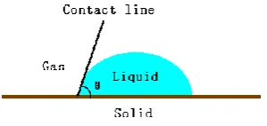
1.4. Dynamic Contact Angle Effects on Liquid Water Transport

Contact angle, which is defined as the angle between the liquid/gas interface and the solid

(17)

4

Figure 1-3 Definition of dynamic contact angle

The value of contact angle is determined by the relationship between three phases (gas, liquid,

and solid), as shown in Table 1-1. When contact angle equals to 0

°

, the solid surface is perfect

wetted. When contact angle equals to 180

°

, then the solid surface is dry, namely perfect

non-wetted. These are the boundaries of contact angle on a flat surface. When the contact angle

is between 0

°

and 90

°

, the surface is hydrophilic, which means liquid tends to be adhesive to the

surface. When the contact angle is greater than 90

°

, the surface is hydrophobic, which means

liquid tends to be repulsive to the surface.

In the equilibrium, contact angle can be expressed by Young’s equation,

⑶

where and are the surface tension of solid/gas interface and solid/liquid interface

respectively [2].

In the case of a droplet resting on a flat surface without shape change, the contact angle is

referred to as static contact angle (SCA) . Before the contact line (between three phases) starts

to move, the maximum of contact angle is the advancing contact angle , while the minimum is

the receding contact angle . These three angles are only in the equilibrium situation.

Table 1-1 Relationship between contact angle and wettability

Contact angle Wettability Shape of droplet

(18)

5

0 < θ < 90° hydrophilic

90° ≤ θ < 180° hydrophobic

θ = 180° dry

However, from many experiments conducted, the surrounding gas flow is unsteady, resulting in

changing of surface tension between gas and liquid, so the contact angle is unlikely to stay in

equilibrium. This type of contact angle with a moving contact line is defined as dynamic contact

angle (DCA), which is a critical parameter in the boundary of unsteady two-phase flow model,

rather than a property of the surface material itself. In investigating the gas-liquid dynamics in

PEMFC, especially when the geometry of fuel cell size is quite small, namely in a microscopic view,

where surface tension weights much on the gas/liquid distribution and transport, it is not proper

to set SCA as a boundary condition, instead, DCA should be considered.

1.5. Objectives

The objective of this thesis is to investigate gas-liquid phenomena inside the cathode of PEMFCs

with different flow field design, considering the effects of DCA. The numerical study is conducted

by means of volume of fluid (VOF) method to tracking the interface of liquid using FLUENT, which

is a powerful computational fluid dynamics (CFD) software. DCA is introduced to the model

through user defined function (UDF) code with an improvement of the Hoffman function which is

used to account for DCA. The present methodology is validated by comparison with experiments,

and implemented to study the emerging, flooding, drainage process, and detailed gas-liquid

(19)

6

1.6. Outline of Thesis

The present thesis is divided into seven chapters. The content for each chapter are summarized

as below:

Chapter 1: To introduce the fundamental knowledge of fuel cell and proton exchange membrane

fuel cell (PEMFC), illustrate the importance of investigating the gas-liquid phenomena in water

management of PEMFC, and depict dynamic contact angle (DCA) effects on liquid water

transport.

Chapter 2: To make literature reviews on the models of PEMFC and DCA, and address three

problems that need improvement in the end of this chapter.

Chapter 3: To introduce the model used in this work, including VOF method and computation of

DCA. An important improvement of the Hoffman function, which is used to account for DCA in

this model, is presented as well.

Chapter 4: To validate the numerical model. Two experiments carried out by other researchers,

slug flow in a rectangular micro-channel, and glycerine droplet impacting glass, are selected for

comparisons. Similar numerical models are conducted with the same geometry and operating

conditions as the experiments, by using presented methodology in this work.

Chapter 5: To investigate gas-liquid phenomena in the cathode of PEMFC with parallel flow field

design. Two cases are conducted using VOF model; one is to apply DCA on multiple wall

boundaries, the other is without DCA, namely using static contact angle (SCA). The results for

each case and comparisons between two cases are described.

Chapter 6: To investigate gas-liquid phenomena in the cathode of the PEMFC with stirred tank

reactor (STR) design. Similar to Chapter 5, two cases with/without DCA are conducted. Results

and comparisons between two cases are described.

(20)

7

2. LITERATURE REVIEW

As a critical research topic for optimizing the performance of PEMFCs, liquid water management

is attracting great efforts from many scientists and engineers [3]. During last two decades, a great

number of research works have been reported by scholars and academic researchers. Singh et al..

[4] developed a two-dimensional model to investigate the transport process in PEMFCs to

improve water management. Previously reported analyses by Djilali and Lu [5] also studied the

influence of heat and water transport in PEMFCs. A three-dimensional numerical model of

straight gas-flow channels was studied by Dutta et al.. [6]. Cha et al.. [7] discussed the influence

of oxygen concentration along gas flow channels on PEMFC performance by examining the

steady-state gas-flow phenomena in micro parallel flow channels. Kulikovsky [8] numerically

acquired the gas concentration of a steady-state flow along channels in a similar way. These

studies, however, did not investigate the influence of liquid water. Yi et al. [9] indicated that water

vapor condensation is a common phenomenon on both sides of a PEMFC. You and Liu [10]

pointed out that a multi-phase model must be employed in order to obtain more practical results.

Both of these previous studies considered water in vapor form [9, 10]. Wang et al. [11] conducted

a two-phase, multi-component mixture model of the cathode of a PEMFC to deal with the

problems in a single- and in a two-phase co-existence region, and introduced a technique to

measure in situ water distribution [12]. Recently, Dawes et al. [13] investigated the effects of

water with a three-dimensional mixture model of a PEMFC, and Luo et al. [14] also developed a

topologically equivalent pore network model to study the transport of liquid water in PEMFC.

These contributions to investigating the water management in PEMFC are summarized by some

review papers. Wang [15] provided a review of fundamental models for PEMFC, and Weber et al..

[16] gave a review of modeling transport. Li et al. [17] outlined progress and achievements of

water management investigation in PEMFC, particularly concentrating on water flooding issues.

The most recent overview was detailed summarized by Jiao et al. [3].

From one-dimensional to multi-dimensional, from single phase to multi-phase, many numerical

models were developed based on computational fluid dynamics (CFD) approaches. Two fluid

model [18-20] and mixture model [21-23] were considered close to the real two-phase flow in a

(21)

8

cathode of PEMFCs. However, these two models are difficult to simulate detailed liquid water

transport. Thus, the volume of fluid (VOF) model was proposed by Quan et al. [24] to simulate

the liquid water removal process by tracking the interface between liquid and gaseous phases.

By means of the VOF model, between 2006 and 2008, a series of numerical simulations of

two-phase flow in several different types of cathode flow field design were conducted [25-29].

The water removal characteristics [25-27], the effects of electrode wettability on liquid water

behaviour [28], and accelerated numerical test of liquid behaviour [29] were investigated, but

neither conventional porous layers nor electrochemical reactions were included in these analyses.

In 2008, a general model for PEMFC has been proposed [30] and applied in the following years

to investigate two-phase flow coupled with electrochemical reactions, water transport through

the membrane, and heat and mass transfer for single cells with different flow field designs [30,

31] and a 3-cell stack [32]. However, this technique requires excessive computational time. In

order to minimize computational time, a simplified model [33] was developed by neglecting

electrochemical reactions and heat transfer effects since computational results were hardly

affected for the aim of simulating liquid water transport. And detailed experimental validation

[33] was performed by direct optical visualization method to capture the motion and

deformation of liquid water. Then liquid water emerging and flooding process inside a PEMFC

cathode with straight parallel [34] and interdigitated [35] flow field designs were studied by

means of this validated simplified model.

All the studies with VOF model mentioned above [24-34] are implemented with static contact

angles on the wall boundaries. The contact angle is determined by the liquid-gas interface on a

solid material, changing with the moving contact line. Djilali et al. [36, 37] noted that liquid water

behaviour on a gas diffusion layer (GDL) surface is affected by the contact angle when water

emerges from a pore, and conducted validation experiments by observation method [38].

Therefore, it is not proper to use static contact angles as a wall boundary condition for the

unsteady, two-phase flow model of the cathode of PEMFC.

Sikalo et al. [39] investigated DCA of spreading droplet using VOF model, through both numerical

(22)

9

compute DCA. He also presents a widely used formula describing the relationship between DCA

and the contact angle in equilibrium. However, they are not dependent on the actual flow field.

Therefore, Sikalo considered the correlation proposed by Kistler [42] which is an application of

Hoffman function. Miller [43] used this method which is best fit to existing experiment results,

and developed a user defined function (UDF) code for pursuing the movements of a droplet in a

single straight channel with implement of DCA on the boundary condition. All models conducted

with DCA so far are in simple geometry domains, usually considering only one boundary with

DCA. Moreover, the DCA values were not extracted within a specific time and location.

To summarize the literature review, some key points can be addressed as follows:

(1) Compared with existing numerical models to study the gas-liquid dynamics in the cathode of

PEMFC, VOF model has the advantage of tracking interface between liquid and gas so that

the liquid water distribution and transport can be described in details. However, most of the

simulation of PEMFC cathode using VOF model have not considered DCA as wall boundaries.

(2) Although many researchers studied the contact angle effects on gas-liquid dynamics and

proposed many correlations to account for DCA, most of models are not dependent on actual

flow field. The method with application of Hoffman function is considered as the best fitting

of experiment results, and good for depicting DCA depending on real flow field.

(3) Some researchers use Hoffman function in their flow model; however, nearly all these

models are simple geometry, usually a straight channel or a plate, and couple DCA only on a

single wall boundary. No one has applied this method on the model of PEMFC cathode with

complex flow field design to investigate the liquid water transport.

In present work, all issues proposed above are solved. The methodology is going to be presented

and validated by comparison with selected experiments. By use of this method, the gas-liquid

phenomena with/without DCA in the cathode of PEMFC with complex flow field, i.e., parallel

design, and stirred tank reactor (STR) design developed by Benziger et al. [44] and Hogarth and

(23)

10

3. NUMERICAL METHODOLOGY

3.1. Brief Model Description

According to the work of Sikalo et al. [39] and Miller [43], and the validated VOF method [23-25],

with an improvement of Hoffman function, a numerical model are developed by implementation

of DCA on multiple wall boundaries through a UDF code.

The numerical model of PEMFC cathode is 3-dimensional, unsteady, two-phase flow, solved by

use of FLUENT software, which is a powerful engineering tool to solve CFD problems. Air is

treated as the gaseous phase while liquid water is treated as the liquid phase, and these

two-phases are assumed to be immiscible. VOF method is applied to track the liquid-gas flow

interface. A UDF code is applied to introduce the source term, apply DCA to multiple wall

boundaries, and extract analytic parameter values, such as liquid water amount, interface

pressure, and local DCA.

The fluid flow is laminar because of the low flow velocity and the small size of the channels. Heat

transfer and phase change are not considered in this study in order to reduce the computation

time. The unsteady, laminar flow model is governed by the following continuity (mass) and

momentum equations to describe the fluid flow transport process.

3.2. Governing Equations and Volume of Fluid (VOF) Method

The continuity (mass) equation is expressed as

ερ

ερ ⑷

where ε is the porosity of the porous media (in the gas flow channels ε ). The first term

on the left hand side is the transient term representing the change of mass with time, the second

term is the convection term standing for the change in mass flux, and the term on the right hand

side is the mass source term. In this study, equals to zero because phase changes are not

taken into account in this model.

In the VOF model, the volume fractions of gas and liquid water are defined as and

(24)

11

⑸

The variables and properties are shared by both phases and are calculated by a volume-averaged

method. The average density and viscosity for each computational cell which is between those of

gaseous and liquid phases, are defined as

ρ ρ ρ ⑹

and

⑺

In the VOF model, the interface between gaseous and liquid phases is tracked by solving a

continuity equation for the volume fraction of liquid water,

ε ρ

ε ρ ⑻

which is solved over the entire computational domain. Then the volume fraction of gas is

computed based on the Equation (5).

A single momentum equation is implemented in the VOF model, and the gaseous phase and the

liquid phase share the same resulting velocity field,

ερ ερ εμ ε ⑼

In this momentum equation, the terms on the left hand side represents the change of

momentum with time and the advection momentum flux respectively, while the terms on the

right hand side are the momentum due to pressure, viscosity and sources.

In the model, the surface tension force, as well as gravity force, is coupled to the momentum

equation by the source term , expressed as

ρ _ρρ_ρ ⑽

(25)

12

In the porous layer, one more term μ_α , where α stands for the permeability of the porous

layer, is added in the source term because of the viscous effect through the porous layer, or the

Darcy force. So the complete source term for the momentum equation in the porous layer is

_ρρ_ρ μ_α ⑾

3.3. Implementation of Dynamic Contact Angle

Dynamic contact angle is implemented in this model by means of compiling the UDF code to the

wall boundary conditions, which is developed based on the empirical expressions contributed by

Kistler [42] and the work of Sikalo et al. [39] and Miller [43],

⑿

The dynamic contact angle is determined by the Hoffmann function , and varies

according to the capillary number and a shift factor gained from the inverse of the

Hoffman function under equilibrium when the contact angle on the wall boundary is fixed,

namely, static contact angle (SCA) [39], i.e.,

⒀

The capillary number , which shows a relationship between viscosity and surface tension

, affected by the contact line velocity which is extracted instantaneously from the model during

iteration, is defined as

⒁

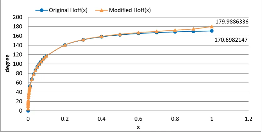
3.4. Improvement of Hoffman Function

The Hoffman function (Equation (13)) is an empirical formula derived through experiments [46].

It is noticed that, in all of these experiments, the shift factor , whose range of value is between

0 and 1 since it is a proportion parameter, was obtained for corresponding contact angels

between 15

°

and 120

°

. This means the applicability of the Hoffman function with a contact angle

(26)

13

During the current investigation, the Hoffman function (Equation (13)) was found to be imprecise.

The value of was found to be greater than 1, that is beyond the upper limit of proportional

parameter value range, with a corresponding contact angle within the range of (171

°

, 180

°

).

Therefore, a correction term is added to the original Hoffman function to improve the

applicability. The revised Hoffman function is expressed as

⒂

A comparative plot with both the original and revised Hoffman functions is presented in Figure

3-1, from which it can be seen that the revised Hoffman function has a wider range of

applicability in the numerical simulation. Consequently, the UDF code implemented the revised

Hoffman function to compute DCAs for specific wall conditions with different SCA in equilibrium

and compile them to this 3-D, unsteady model.

Figure 3-1 The calculated values of original and revised Hoffman function 170.6982147 179.9886336 0 20 40 60 80 100 120 140 160 180 200

0 0.2 0.4 0.6 0.8 1 1.2

d e gr e e x

(27)

14

4. NUMERICAL MODEL VALIDATIONS

4.1. Volume of Fluid (VOF) Method Validation

A simplified VOF model, in which electrochemical reactions and heat transfer effects were

neglected to minimize the computational time, is validated by Le et al. [33]. Numerical simulation

was used to predict the liquid water behaviours in the cathode of a PEMFC with serpentine

channels and a porous layer. A detailed experimental validation of this simplified cathode model

was performed by direct optical visualization method to capture the motion and deformation of

liquid water with high spatial and temporal resolutions. A sample comparison from this validation

is shown in Figure 4-1 (the left panel shows the experimental setup, while the right panel shows the

numerical simulation), which demonstrates that the results from this simplified model are in good

agreement with the corresponding experiments.

Figure 4-1 Comparison of liquid water behaviours between numerical simulation and the experiment at t = 0.400s [33]

4.2. Dynamic Contact Angle Methodology Validations

Two interesting experiments were selected for the validation of the present model with DCA

coupling on wall boundary conditions. One was conducted by Fang et al. [47], who studied slug

flow in a micro-channel; the other was carried out by Sikalo and Ganic [40] and Sikalo et al. [41],

which was impact of a droplet on glass. In order to validate the methodology proposed in this

(28)

15

under the same conditions with the experiments. Detailed validated cases are presented, and the

comparisons of results between numerical and experimental models are addressed in the

following section.

4.2.1. Slug Flow in Rectangular Micro-channel

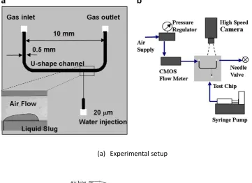
4.2.1.1. Brief Description

Fang et al. [47] conducted experiments of liquid slug flow in micro-channels with several of input

parameters. The schematic of the experimental setup is shown in Figure 4-2(1). The test bench is

a 10 mm long, 0.5 mm wide U-shape micro-channel made of silicon. A three-dimensional,

two-phase flow model of this experiment also using VOF theory was validated by Fang et al. [47].

The computational domain is shown in Figure 4-2(2), which is a straight channel with 5 mm in

length and has a cross-section of 500 μm × 45 μm. Air is supplied to the inlet boundary of

the channel as gaseous phase with a constant velocity of 15.56 ms-1, while liquid water is supplied to the liquid inlet boundary, which is located at one third of the length from the air inlet,

as liquid phase with a constant velocity of 0.09 ms-1. The initial contact angle on the bottom wall of the channel is 105

°

. DCA was implemented on the wall boundary as well, but in the

computational manner differing from the methodology presented in this thesis. The experimental

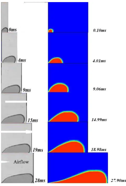
and numerical results supplied by Fang et al. [47] are shown in Figure 4-2(c) (gas is coloured in

blue, and liquid is coloured in red).

The methodology presented in this thesis has the advantage of plotting local contact angle with

time (i.e. DCA field) compared to Fang’s model. In order to validate the present methodology, a

numerical model with same dimensions and operating parameters but different way of

computing and compiling DCA to the wall boundary is conducted. Both air and liquid water are

(29)

16

(a) Experimental setup

(b) Numerical model setup

(c) Numerical (first row) and experimental (second row) results

Figure 4-2 Numerical and experimental slug flow model conducted by Fang et al. [46]

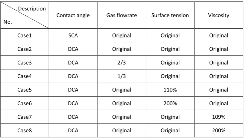
4.2.1.2. Validation

Figure 4-3 shows comparison of results between Fang’s experiments and the present numerical

(30)

17

similar, but the time directions in the two models are hard to fit well. In order to investigate the

potential factors that influence the comparison, a series of slug flow testing cases with changes of

parameters were conducted with descriptions as in Table 4-1. These cases will be compared and

discussed by groups in the following section.

Figure 4-3 Results comparison between Case2 (second row) and experiment (first row)

Table 4-1 Description of conducted cases in numerical slug flow model

Description

No.

Contact angle Gas flowrate Surface tension Viscosity

Case1 SCA Original Original Original

Case2 DCA Original Original Original

Case3 DCA 2/3 Original Original

Case4 DCA 1/3 Original Original

Case5 DCA Original 110% Original

Case6 DCA Original 200% Original

Case7 DCA Original Original 109%

Case8 DCA Original Original 200%

(31)

18

presented entirely so that some phenomena might be neglected. Therefore, the gas flowrate may be the factor affecting the validation results.

Figure 4-4 Results comparison between Case4 and experiment

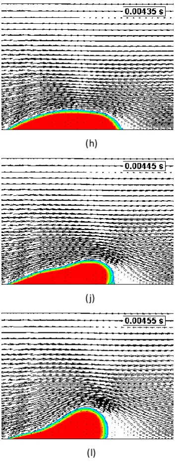
Since the provided experimental results are fragmentary, the whole movement cannot be tracked

from Fang’s paper. Whereas, an interesting worm crawling phenomenon of liquid water can be

observed periodically in the numerical model with DCA implementation (Case2) (as shown in

Figure 4-5). This phenomenon divides into accumulation, flattening, re-accumulation; three

sub-processes caused by a cooperation of pressure, surface tension, and shear stress. In the

accumulation sub-process (Figure 4-5(a, b)), surface water in the slug is driven by the air flow,

and the head of slug is held by the surface tension. The air flow converges and increases the

velocities in the windward side of the water slug resulting in a high pressure area; while the

velocities at the leeward of the slug decreases forming a low pressure area. This pressure drop in

(32)

19

The pressure between the two sides decreases. With surface of the water slug increasing, the

surface tension increases as well. So the slug recedes a little bit as shown in Figure 4-5(h-l), and

then re-accumulates. The worm crawling phenomenon reveals the interaction between the two

phases, i.e., gas and liquid water. The different slug shape at difference time instances

corresponds to the relationship between pressure, surface tension, and shear stress at specific

time instance.

(a) (b)

(c) (d)

(33)

20

(g) (h)

(i) (j)

(k) (l)

(m)

(34)

21

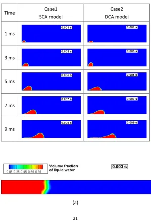
4.2.1.3. Dynamic Contact Angle Effects

The numerical model with contact angle fixed, namely SCA (Case1), is conducted with other

settings identical to the DCA case (Case2). The comparison of results between Case1 and Case2

are presented in Table 4-2. It can be noticed that the contact line between gas and water in Case1

is held at a steady angle, which violates the physics of slug motion. Since the velocities near the

contact line change in magnitude and/or direction over time, the contact angle on the bottom

wall should alter correspondingly, which affects the water transport in contrary because of

changes in wall adhesion. Figure 4-6 shows the water distribution on the wall with corresponding

DCAs at 0.03 s. The area where volume fraction of water shifts intensely has a large DCA

difference because of the greater change of velocity.

Table 4-2 DCA effects on the slug flow model

Time Case1 SCA model

Case2 DCA model

1 ms

3 ms

5 ms

7 ms

9 ms

(35)

22

(b)

Figure 4-6 (a-b) Liquid distribution with DCA on the bottom wall in Case2

4.2.1.4. Mass Flowrate, Surface Tension, and Viscosity Effects

The effects of gas mass flowrate are studied by conducting the numerical model with 1/3

percentage decrease gradually. Case 3 is the numerical model with 2/3 of original air mass

flowrate, and Case 4 is the one with 1/3 of original air mass flowrate. These two cases are

compared with the original air flowrate (Case2), shown in Table 4-3. All three cases are

conducted with DCA implementation. From the results in Table 4-3, lower air mass flowrate leads

to a longer time when water slug is stuck at the liquid inlet.

Table 4-3 Air mass flowrate effects on the slug flow model

Time Case2 Original DCA model

Case3 2/3 air mass flowrate

Case4 1/3 air mass flowrate

1 ms

3 ms

5 ms

7 ms

9 ms

Similarly, two cases with increase of surface tension are conducted and compared with the

(36)

23

increase of 100%. From the comparison in Table 4-4, it can be noticed that with higher surface

tension the slug prefers to be held near the liquid inlet field.

Table 4-4 Surface tension effects on the slug flow model

Case5 110% surface tension

Case6 200% surface tension

1 ms

3 ms

5 ms

7 ms

9 ms

To study the effect of viscosity, Case7 has an increase of 9% and Case8 has an increase of 100%.

Unlike previous groups with changing of air flowrate and surface tension, the change of viscosity

does not have much influence on the transport of slug flow, with only slight altering in the shape,

in other words, viscosity slightly affects the interaction of the two phases.

Table 4-5 Viscosity effects on the slug flow model

(37)

24

7 ms

9 ms

4.2.2. Impact of Droplet on Smooth Glass

4.2.2.1. Brief Description

Since the validation methodology is not reliable by comparing only to one experiment, another

experiment was selected for the validation of the present model. Sikalo and Ganic [40] and Sikalo

et al. [41] conducted a series of experiments of droplet impacting on a plate with different

droplet and surface materials, and impact velocity given in Weber number. The experimental

setup used by these researchers is shown in Figure 4-7.

Figure 4-7 Experimental setup for droplet impact model [41]

One of the experiments was selected for validation of the present methodology in this thesis,

which is an impact of glycerine droplet on a horizontal glass plate. The initial diameter of

(38)

25

Weber number is 391, which give a velocity of 3.635 ms-1.

By sharing the same setting as in the experiment, a numerical model has been developed using

the simplified VOF model, considering the DCA effects by compiling the UDF code on the wall

boundary (which is glass in this model), for the sake of methodology validation. Another model,

with only difference of fixing the contact angle on the wall (i.e., SCA), is conducted for

comparison as well. The geometry of the numerical model is a cylinder with dimensions of 10

mm diameter and 4.0 mm height, with implementation of pressure-inlet boundary on the surface

to simulate the surrounding atmosphere. The initial setting of contact angle on the glass (which is

wall boundary) is 15

°

. The mesh size for this numerical model is 0.2 mm. Grid independency is

determined by deducting 50% of the mesh size and the differences of results are very small.

4.2.2.2. Comparisons

Figure 4-8(a) is the experimental results from Sikalo and Ganic [40] captured by CCD camera at

0.100, 0.260, and 2.020 ms (the latest three profiles of droplet) with the starting time (0 s) at the

moment of impact. The results of the numerical model with/without DCA effects are shown in

Figure 4-8(b, c) with same dimension scales and time difference, in which the starting time is 0.4

ms earlier than that in experiments. Comparing the results from the three models, the results are

similar between each other. Both the DCA and SCA models can simulate the experimental results

well.

(a) Experimental model (b) SCA model (c) DCA model

Figure 4-8(a-c) Results comparison of droplet impact model (a)Experimental results at 0.100, 0.260, 2.020ms [40]

(b, c) Numerical results at 0.500, 0.650, and 2.420 ms (time direction with 0.4ms difference with experiments)

(39)

26

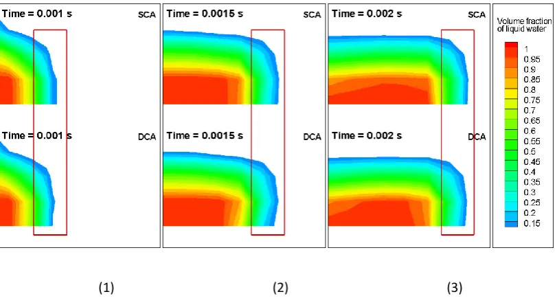
small difference, as shown in Figure 4-9, which illustrate an enlarged part of glycerine droplet

spreading on the glass at 0.001s, 0.0015s, and 0.002s. By reference of marking rectangle in the

figure, it can be observed that the joint of glycerine droplet and glass are slightly different.

Compared to SCA model, the results in DCA model are closer to the experimental results as

shown in Figure 4-10 which is an enlarged view of Figure 4-8(a).

(1) (2) (3)

Figure 4-9 Results comparison between SCA and DCA model of glycerine impact

(40)

27

4.2.2.3. Dimple Phenomenon

When the glycerine droplet falls, the potential energy is converted to kinetic energy. When the

droplet impacts the glass plate, its momentum alters greatly, both in magnitude and direction, so

the droplet spreads on the glass. Because of the conservation of mass, there is no more glycerine

supplied in the middle area, while the rim of the droplet is continuously spreading. Then the

dimple phenomenon happens on the surface of the impacting droplet (Figure 4-11(a)). Figure

4-11(b) shows the corresponding DCAs (by cutting off the values of 15

°

(initial contact angle) and

below) on the glass at the same time instance. In the middle area, the contact angles are smaller

than other impacting areas revealing the strong hydrophilic wettability of these areas on the glass.

Also the DCAs are much higher in the rim of the droplet, which demonstrates the intensive

movement of glycerine there.

(a) (b)

Figure 4-11(a-b) Depression phenomenon (liquid volume fraction with corresponding DCA on the glass at 0.002424 s)

4.3. Summary

The validation of the numerical methodology of VOF model with implementation of DCA is

processed by conducting two series of models to compare the numerical results with

experimental results. Two experiments, one is a water slug flow in a straight channel, the other is

a glycerine droplet impact on glass, are selected for numerical model validation. For slug flow in a

channel, numerical results partially fit experimental results; some potential factors affecting the

results comparison exist. For the glycerine droplet impact on a glass plate, the numerical results

(41)

28

5. GAS-LIQUID PHENOMENA IN PROTON EXCHANGE MEMBRANE FUEL

CELLS WITH PARALLEL DESIGN

5.1. Numerical Model Setup

As one of the major flow channel designs, parallel channels permit a low overall pressure drop

between the gas inlet and the outlet [48]. Two numerical models, Parallel-SCA and Parallel-DCA,

which share the same computational domain and operating conditions but with only difference

on wall boundaries, are implemented in order to investigate the liquid water transport within this

type of channel design by considering of DCA effects.

5.1.1. Geometry Domain

The numerical simulation domain for the parallel model represents a full-scale cathode side

geometry of a single PEMFC. Figure 5-1 illustrates the schematic of the numerical simulation

domain, which contains gas flow channels, including seven parallel channels with a 0.001 m

distance between adjacent ones, and a porous layer whose porosity is 0.3. The dimensions of the

entire computational domain are 0.06 m in X-direction, 0.024 m in Y-direction, and 0.002 m in

Z-direction. The cross-section of the parallel channels is 0.002 m (in X-direction) × 0.002 m (in

Y-direction) × 0.0017 m (in Z-direction). Main part of gas flow channels are attached to a 0.024

m (in X-direction) × 0.024 m (in Y-direction) × 0.0003 m (in Z-direction) porous layer with

0.002m frames on X-Y plane. These are the typical dimensions of a fuel cell component. A liquid

water injection channel (LWIC) with dimensions of 0.0004 m (in X-direction) × 0.0004 m (in

Y-direction) × 0.000725 m (in Z-direction) is positioned at the inlet joint (the joint of inlet

channel and No.1 parallel channel) shown in Figure 5-1. This LWIC was used to simulate liquid

water injection effects in previous studies [33]. In the present parallel model, the LWIC is blocked

because there is no liquid water injected through it, and this geometry is kept so that the results

of the current study (where the liquid water is supplied from the back surface of the porous layer

as shown in Figure 5-1) can be compared to the results of previous studies (where liquid water

injection is performed through the LWIC) in the future. The direction of gravity is along negative

(42)

29

Figure 5-1 Computational domain of Parallel model

5.1.2. Boundary Conditions

The computational methodology is applied in the parallel model by means of specific boundary

conditions as shown in Table 5-1. In Parallel-SCA model, initial contact angles for wall boundaries

are fixed as constant; while in Parallel-DCA model, contact angles change with the change of flow

field (i.e., dynamic contact angle (DCA)) during simulation through the UDF code coupling on the

wall boundaries, and can be expressed as parameters associated with time and location.

Table 5-1 Boundary conditions of the parallel model

Boundaries Type Descriptions

Liquid inlet

(Back surface of porous layer) Mass flow inlet Mass flowrate: 1.7×10

4

kgs-1

Gas inlet Mass flow inlet Mass flowrate: 2.0×10-5 kgs-1 Outlet Pressure outlet Pressure: 1 atm

Walls

Side walls of

channels Wall No-slip, initial contact angle: 40° Upper walls of

channels Wall No-slip, initial contact angle: 43° Walls of porous layer

(walls under frames and lands)

(43)

30

5.1.3. Grid Independency

The computational domain is meshed with 290,352 cells in total. The cell size is approximately

1.67×10-4 m in both X- and Y-directions, whereas the dimensions in Z-direction are 1.4×10-4 m in the gas flow channel domain and 5×10-5 m in the porous layer domain. Jiao et al. [26] implemented a grid check method by increasing and decreasing the number of grid cells by

certain percentages. This cell size has been validated for PEMFCs by the comparison of numerical

results with experimental results from the previous studies [33].

5.2. Liquid Water Transport in Parallel Model without Dynamic Contact Angle

5.2.1. General Process

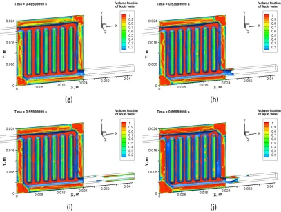
Figure 5-2 shows the main process of liquid water movement over time for some selected time

instants, where volume fraction of liquid water is expressed by colour-filled contours with

iso-surface. The general process of liquid water transport can be divided into the following

sub-processes:

(1) Liquid water is supplied from the back surface of the porous layer by a constant mass

flowrate to simulate the liquid water generation through electrochemical reaction (Figure

5-2(a)).

(2) This supplied liquid water mounts up in the porous layer (Figure 5-2(b-d)), and reaches the

top surface of the porous layer, i.e., the interface between the porous layer and channels,

first at four corners of the interface under the channels domain (Figure 5-2(b)), then frame

(Figure 5-2(c)), and also the edges of each parallel channel (Figure 5-2(d)).

(3) Liquid water from the porous layer emerges into the gas flow channels from the peripheral

edges of lands (defined as the solid between adjacent parallel channels on bipolar plate) and

the peripheral edges of the channels domain (Figure 5-2(e-f)).

(4) The liquid water emerging into the channels accumulates at the outlet joint (defined in

Figure 5-1) (Figure 5-2(g)).

(44)

31

(6) Liquid water drains out through the outlet channel (Figure 5-2(i)). With liquid water

increasing, some parts of the gas flow channels get flooded, and the second draining

process happens (Figure 5-2(j)).

(a) (b)

(c) (d)

(45)

32

(g) (h)

(i) (j)

Figure 5-2(a-j) General liquid water transport in Parallel-SCA model

5.2.2. Emerging Process

5.2.2.1. Liquid Water Emerging from Peripheral Areas of Lands and Frames

As shown in Figure 5-3, two planes are extracted near the interface (Z = 0.00029 m and Z =

0.00031 m), from the porous layer domain (left column in Figure 5-3) and channel domain (right

column in Figure 5-3) respectively, to explain the pattern of liquid water emerging into the gas

flow channels from the porous layer. From Figure 5-3(a-1), it can be noticed that liquid water

initially reaches the interface under peripheral edges of the channel domain, and tends to

accumulate under the area of edges of lands (the ribs between two adjacent parallel channels as

defined in Figure 5-1). At the same time instance, liquid water already enters into the gas flow

channels from the peripheral edges of the channel domain (Figure 5-3(a-2)). Soon after, liquid

water emerges from the edges of lands (Figure 5-3(b-2)), meanwhile the areas underneath the

lands in the porous layer domain are filled with liquid water (Figure 5-3(b-1)). As time goes by,

more liquid water is generated, passes through the interface, and enters into the channels (Figure

(46)

33

The detailed emergence and growth of liquid water from the porous layer into channels can be

explained by Figure 5-5. The left column in Figure 5-5 shows the liquid water volume fraction on

the plane extracted from computational domain at Y = 0.012 m (Figure 5-4); and the right column

is the enlarged area of No. 7 parallel channel on the plane, showing velocity as well as volume

fraction with different reference velocity vectors. The liquid water from the porous layer enters

into the channels from the edges of the lands because the liquid water generation rate is uniform

on the back surface of the porous layer, but the liquid water underneath the lands cannot directly

enter into the channels in the manner that the liquid water underneath the middle of the

channels enters. Actually, the liquid water underneath the lands has to detour along the interface

between the lands and the porous layer then into the channels because the lands are solid and

only allow the conduction of electrons.

(a-1) (a-2)

(47)

34

(c-1) (c-2)

Figure 5-3(a-c) Liquid water distribution near interface in Parallel-SCA model (Left column: plane at Z = 0.00029 m; right column: plane at Z= 0.0031 m)

Figure 5-4 Extract a plane from Parallel computational domain at Y=0.0012m

(48)

35

(b-1) (b-2)

(c-1) (c-2)

Figure 5-5(a-c) Emerging process on plane at Y = 0.012 m in the Parallel-SCA model (Left column: entire plane; right column: enlarged plane with velocity (the upper reference vector

is in No. 7 parallel channel, and the lower reference vector is in the porous layer))

5.2.2.2. Dean Vortex Evolution

For the X–Z plane at Y = 0.012 m (Figure 5-5), it can be noticed that there are a pair of vortices –

an upper vortex and a lower one – in the cross-section of the parallel channels, referred to as

Dean vortices, which occurs in curved channels or pipes [49]. This tangential flow enhances the

ability of liquid water removal along the primary direction of gas flow channels. Because of the

effects of Dean Vortices and gravity, the emerged liquid water occupies the lower corners of the

channel cross-section, attaches to the sidewalls due to wall adhesion, and gets removed by the

primary gas flow. It can also be noticed that the emergence of liquid water affects the gas flow

pattern. Especially in Figure 5-5(a-2), when liquid water first enters into the channel from the

right corner in the cross-section, Dean vortices are distorted with approximately 45

°

in

anti-clockwise direction. This interesting phenomenon shows the interaction between gaseous

(49)

36

5.2.3. Draining Process in Outlet Channel

The draining process in the Parallel-SCA model can be explained by Figure 5-6, showing the

deformation of draining liquid water in the outlet channel. The liquid water coming from the

porous layer near the peripheral zones of the four frames and the lands gradually develops into

two liquid water streams, with the first stream accumulating at the bottom of the outlet manifold

and the second stream accumulating on the side wall of No. 7 parallel channel. These two

streams meet near the outlet joint and gradually form a valley shape (Figure 5-6(1)). This shape is

formed due to the combined effects of wall adhesion and liquid water surface tension. At the

same time, the air streams from all directions also meet and merge into one stream at the outlet

joint; this combined air stream continuously strikes the windward side of the valley shape, forcing

it to move along the outlet channel and be more sharp (Figure 5-6(b)). Then, this valley shaped

water deforms into a top–bottom stratified flow pattern while moving along the outlet channel

to drain (Figure 5-6(c-h)). Several splashed small droplets are not removed together with the

top–bottom stratified flow but adhere to the sidewalls of outlet channel; that is because their

inertial force is not strong enough to overcome the friction or wall adhesion. These liquid water

removal processes repeat for a period of time, similar deformation occurs for each draining

period.

(a) (b)

Gas-liquid phenomena with dynamic contact angle in cathode of proton exchange membrane fuel cells

Scholarship at UWindsor

Scholarship at UWindsor

Gas-liquid phenomena with dynamic contact angle in cathode of

Gas-liquid phenomena with dynamic contact angle in cathode of

proton exchange membrane fuel cells

proton exchange membrane fuel cells

GAS-LIQUID PHENOMENA WITH DYNAMIC CONTACT ANGLE IN

CATHODE OF PROTON EXCHANGE MEMBRANE FUEL CELLS

by

XICHEN WANG

A Thesis

Submitted to the Faculty of Graduate Studies

through Mechanical, Automotive and Materials Engineering

in Partial Fulfillment of the Requirements for

the Degree of Master of Applied Science at the

University of Windsor

Windsor, Ontario, Canada

2011

Gas-liquid phenomena with dynamic contact angle in cathode of proton exchange

membrane fuel cells

by

Xichen Wang

APPROVED BY:

______________________________________________

Dr. Tirupati Bolisetti

Department of Civil & Environmental Engineering

______________________________________________

Dr. Ronald M Barron

Department of Mechanical, Automotive & Materials Engineering

______________________________________________

Dr. Biao Zhou, Advisor

Department of Mechanical, Automotive & Materials Engineering

______________________________________________

Dr. Amir Fartaj, Chair of Defense

Department of Mechanical, Automotive & Materials Engineering

DECLARATION OF PREVIOUS PUBLICATION

ABSTRACT

DEDICATION

ACKNOWLEDGEMENTS

TABLE OF CONTENTS

LIST OF FIGURES

LIST OF TABLES

NOMENCLATURE

Density (kgm

)

Porosity

Velocity vector (ms

)

Source term

Phase volume fraction

Surface tension coefficient

Surface curvature (m

)

Permeability (m

)

Dynamic contact angle (°)

Contact angle in equilibrium (°)

Capillary number

Hoffmann function

Inversed Hoffmann function

Improved Hoffmann function

Shift factor

Dynamic viscosity (Pas)

Surface tension (Nm

)

Contact line velocity (ms

)

Subscripts

Gas phase

Liquid phase

Continuity (mass) equation

1.

INTRODUCTION

°

°

°

°

°

2.

₎