Design of a 50 GHz Bandwidth DPSK Compatible Monolithically Integrated Optical Receiver

(1)

ABSTRACT

BOGACKI, KEVIN JOSEPH. Design of a 50 GHz Bandwidth DPSK Compatible Monolithically Integrated Optical Receiver. (Under the direction of Dr. Leda Lunardi.)

The goal of this work is the design, analysis, and simulation of a monolithic optical

receiver consisting of two balanced waveguide photodiodes integrated with a differential

transimpedance amplifier, based on InP double heterojunction bipolar technology for 50 Gb/s

differential phase shift keying (DPSK) applications.

For the InP / InGaAs double-heterojunction bipolar transistor (DHBT), a small signal

equivalent model based upon the Gummel-Poon bipolar junction transistor model was used.

This model was determined by fitting measured S-parameters from a published 180 nm

collector base-metal-overlaid structure (BMOSA) with a 20 μm2 hexagonal emitter area. In addition, a thermal model was incorporated to estimate the device operating temperatures.

The maximum cut off frequency and maximum frequency of oscillation of the model were

289 and 210 GHz, respectively.

For the InGaAs PIN waveguide photodiode (PIN-WGPD), a small signal equivalent

model was also developed based upon published data. The model parameters were found by

fitting the photodiode gain profile to measured results for a 300 nm thick evanescently

waveguide coupled PIN-PD with a 5x20 μm2 _{total area. The bandwidth of the photodiode}

was 70 GHz with a corresponding responsivity value of 0.37 A/W.

With the transistor model, a fully differential 3-stage transimpedance amplifier was

designed. The optimized amplifier yielded a gain of 18.8 dB, bandwidth of 50.3 GHz,

(2)

of 28.8 dB. DC simulations indicated that all devices operated at a temperature of less than

144oC, while total power dissipation was less than 305 mW.

Finally, the optimization of the fully integrated optical receiver was evaluated. Two

integration schemes were investigated – hybrid and monolithically integrated – with the

monolithic optical receiver outperforming the hybrid architecture in terms of wider

bandwidth and faster performance. The monolithic receiver showed a gain of 14.3 dB and a

bandwidth of 50.0 GHz with input and output reflections better than -10 dB, and exhibited

open eye diagrams at 50 Gb/s in DPSK format with an optical dynamic range of 29.0 dB.

Noise analysis on the monolithic optical receiver yielded an input referred current noise of

(3)

DESIGN OF A 50 GHZ BANDWIDTH DPSK COMPATIBLE MONOLITHICALLY INTEGRATED OPTICAL RECEIVER

by

KEVIN JOSEPH BOGACKI

A thesis submitted to the Graduate Faculty of North Carolina State University

in partial fulfillment of the requirements for the Degree of

Master of Science

ELECTRICAL ENGINEERING

Raleigh, North Carolina

2006

APPROVED BY:

_________________________ _________________________ Dr. D. W. Barlage Dr. Kevin Gard

________________________________ Dr. Leda Lunardi

(4)

BIOGRAPHY

Kevin Joseph Bogacki was born on February 24, 1982 in Rochester, NY. He

graduated high school from Cathedral Prep in Erie, PA with a 4.0 GPA and the Excellence in

English award. He entered Gannon University in 2000 and majored in electrical and

computer engineering. During his tenure at Gannon University, he was the Eta Kappa Nu –

Iota Nu chapter president, an active IEEE student member, and was recognized as the

runner-up for the HKN Norman R. Carson Award for the Outstanding Junior Electrical Engineering

Student in the United States of America. He interned fulltime at Verizon Communications

with the Network Planning and Engineering group and his senior project was the design of a

sensor network for a home security system. In 2004, he graduated summa cum laude and

received the Academic Excellence Award for Electrical and Computer Engineering and the

Archbishop John Mark Gannon Award for General Scholastic Excellence. Kevin then went

on to begin research at North Carolina State University in optical communications under Dr.

Leda Lunardi. Initially, he was sponsored by the NCSU Dean’s fellowship and the Nortel

Networks fellowship, and he worked as an electrical engineering teaching assistant. He then

became a research assistant under Dr. Lunardi and received the Lincoln Laboratory

fellowship from MIT, where he interned for a summer in the Optical Communications

Technology group establishing a 10 Gb/s differential phase shift keying optical

communication link. He is currently a candidate for the degree of Masters in electrical

(5)

ACKNOWLEDGMENTS

This work would not have been possible if not for the guidance and dedication of the

author’s advisor, Dr. Leda Lunardi. Dr. Lunardi provided constant inspiration and

encouragement throughout the author’s master’s work. Although Dr. Lunardi had

responsibilities outside of North Carolina, her amazing commitment to her students at NCSU

brought her back for weekly meetings an allowed her to be only an email or phone call away.

The author would also like to thank Dr. Lunardi for believing in his abilities and always

pushing him towards academic excellence.

The author also thanks Dr. Douglas Barlage and Dr. Kevin Gard for serving on the

advisory committee. Dr. Barlage provided invaluable feedback throughout the author’s work

on device modeling and noise analysis, while Dr. Gard provided his expertise on circuit

design. Furthermore, Dr. Gard’s analog circuit design course and Dr. Barlage’s microwave

engineering course were most beneficial to the author.

Finally, the author would like to thank his family for always being there. Without

their love and encouragement, none of this work would have been achievable. The author’s

parents provided stability and guidance, while his brother and sister provided friendship and

support throughout the author’s academic career and life journeys. For this, the author

dedicates this work to them.

(6)

LIST OF TABLES

Page

Table 2.1 Capacities of current technology……….... 19

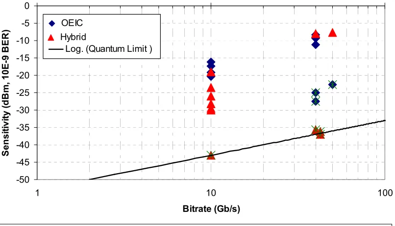
Table 2.2 Experimental receiver sensitivity……… 37

Table 3.1 Optical receiver specification table……… 64

Table 3.2 DHBT layer materials [59]………. 66

Table 3.3 DHBT model parameters……… 68

Table 3.4 Thermal conductivities of selected materials [29]……….. 69

Table 3.5 DHBT self-heating model parameters……… 69

Table 3.6 ft and fmax comparison between simulated model and measured results [59]……….. 72

Table 3.7 DHBT model parameter listing for new 50 GHz bandwidth appropriate model (see text)………... 73

Table 3.8 ft and fmax listing for new 50 GHz bandwidth appropriate model (see text)………. 74

Table 3.9 WGPD layer materials……… 75

Table 3.10 WGPD model parameters………... 76

Table 3.11 Optimum DHBT bias conditions……… 82

Table 3.12 TIA parameter variables………. 94

Table 3.13 TIA parameter variables………. 97

Table 3.14 Bond wire and pad parasitic values [54-55]……… 100

Table 3.15 Discrete optical receiver parameter variables………. 101

Table 3.16 Monolithic optical receiver parameter variables……… 103

Table 4.1 Optical receiver specification and compliance table……….. 104

Table 4.2 TIA Parameter Variables……… 105

Table 4.3 Bias conditions of differential TIA amplifier stages (with single 5V power supply)……… 105

Table 4.4 Bias conditions of TIA bias circuit………. 106

Table 4.5 Dissipated power for TIA………... 106

Table 4.6 Dissipated power for TIA bias circuit……… 107

Table 4.7 Temperature operation of DHBTs in TIA……….. 108

Table 4.8 Differential TIA high frequency comparison of simulated results to Weiner’s measured results [91]………... 110

Table 4.9 Large signal simulations for differential TIA as compared to measured TIA published by Weiner [91]……… 117

Table 4.10 Optical receiver parameter values……….. 117

Table 4.11 Bias conditions of discrete receiver amplifier stages………. 118

Table 4.12 Bias conditions of monolithic receiver amplifier stages………. 118

Table 4.13 Bias conditions of discrete receiver bias circuit………. 119

Table 4.14 Bias conditions of monolithic receiver bias circuit……… 119

Table 4.15 Dissipated power for discrete receiver……… 119

Table 4.16 Dissipated power for monolithic receiver……….. 120

Table 4.17 Dissipated power for discrete receiver bias circuit………... 120

(9)

Table 4.19 Temperature operation of DHBTs in discrete receiver……….. 122 Table 4.20 Temperature operation of DHBTs in monolithic receiver……….. 122 Table 4.21 High frequency comparison of monolithic receiver versus

discrete receiver……….. 124 Table 4.22 Large signal simulations for monolithically integrated receiver

as compared to discrete receiver………. 132 Table 5.1 Monolithic optical receiver parameter values for minimum noise…………. 141 Table 5.2 Bias current / ∆ bias needed to stay within ± 1 pA / Hzof the

noise minimum………... 146 Table 5.3 NF results of monolithic optical receiver optimized for different

(10)

LIST OF FIGURES

Page

Figure 1.1 Optical SNR versus bit-error-rate for DPSK and OOK systems

at 40 Gb/s [96]……… 1

Figure 1.2 Advanced technologies available for high-speed optical communications [36]……….. 2

Figure 2.1 Index profile of step-index fiber with core radius r……… 6

Figure 2.2 Multimode fiber light propagation conditions……… 7

Figure 2.3 Single mode fiber absorption spectrum [33]……….. 11

Figure 2.4 Dispersion versus wavelength for a standard single mode fiber [40]………. 14

Figure 2.5 Chirped optical pulse as a function of time [72]………. 15

Figure 2.6 Basic wave division multiplexing (WDM) setup. This system multiplexes n optical channels, each of X Gb/s, to combine for a total rate of nX Gb/s……… 18

Figure 2.7 A basic modern fiber optic communication link consisting of an optical transmitter, amplifier, and receiver……… 19

Figure 2.8 (a) Simple Fabry-Perot laser diagram (b) Multimode spectral characteristics………. 21

Figure 2.9 (a) Distributed Feedback laser (b) Single-mode spectral characteristics………. 22

Figure 2.10 Basic Mach-Zehnder modulator schematic……….... 25

Figure 2.11 Cross section, schematic top view, and package view of dual drive lithium niobate MZM [97]………. 25

Figure 2.12 Monolithically integrated lumped electrode EAM and DFB laser [86]……… 26

Figure 2.13 Three band energy diagram for EDFA………... 28

Figure 2.14 Gain of typical EDFA as function of wavelength and pump power [72]………... 29

Figure 2.15 Optical spectra and intensity eye diagrams for various modulation formats [93]………. 30

Figure 2.16 Simple RZ-OOK system diagram………... 32

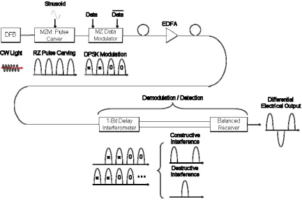
Figure 2.17 Simple RZ-DPSK system diagram………. 34

Figure 2.18 Outline of the optical receiver……… 35

Figure 2.19 Experimental receiver sensitivity……… 38

Figure 2.20 Example eye diagram………. 42

Figure 2.21 Typical 1550 nm photodiode in photoconductive mode [25]………. 43

Figure 2.22 Current-voltage characteristic of a p-n junction [32]………. 45

Figure 2.23 Vertical illuminated photodiode [38]………. 46

(11)

Figure 2.25 Bandwidth versus quantum efficiency tradeoff [6]……… 48

Figure 2.26 Double-pass vertical illuminated photodiode [38]………. 50

Figure 2.27 Vertical illuminated photodiode (b) Waveguide photodiode [38]…………. 50

Figure 2.28 Mushroom-mesa waveguide photodiode [38]……….... 52

Figure 2.29 Bandwidth versus quantum efficiency for the vertically illuminated photodiode and waveguide photodiode [39]………... 52

Figure 2.30 (a) Simple high-impedance front-end amplifier (b) Simple transimpedance front-end amplifier [72]……… 54

Figure 2.31 Advanced technologies available for high optical communication bit rates [85]……… 56

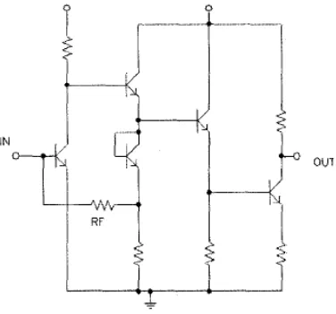
Figure 2.32 Amplifier #1……… 57

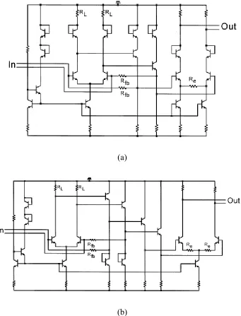
Figure 2.34 Amplifier #3 (a) SiGe implementation (b) InP Implementation……… 59

Figure 2.35 Amplifier #4 (a) HBT implementation (b) HFET implementation………… 60

Figure 2.38 Detailed block diagram of DPSK optical receiver………. 62

Figure 2.39 Discrete DPSK optical receiver and block outline [81]………. 63

Figure 2.40 Monolithic DPSK optical receiver overview [37]……….. 63

Figure 3.1 DPSK receiver block diagram……… 65

Figure 3.2 DHBT device cross section [59]………. 66

Figure 3.3 DHBT model topologies (a) large signal (b) small signal [109]……… 67

Figure 3.4 DHBT self-heating model [109]………. 68

Figure 3.5 DHBT device I-V curves with temperature profile……… 70

Figure 3.6 S-parameter comparison. Measured data taken from [59]………. 71

Figure 3.7 S21 comparison. Measured results taken from [59]………... 71

Figure 3.8 ft and fmax of DHBT model. Measured results taken from (VCE = 1.2 V) [59]……….. 72

Figure 3.9 S-parameter comparison for adjusted model. Measured results taken from [59]……… 74

Figure 3.10 WGPD device cross section………... 75

Figure 3.11 WGPD small signal model topology [60]……….. 76

Figure 3.12 S-parameter comparison. Measured results taken from [88]………. 77

Figure 3.13 Differential transimpedance amplifier topology……… 78

Figure 3.14 ft / fmax curves illustrating proper bias points (note that these curves are the same curves presented Figure 3.8, meaning this is for the original model, not the adjusted model. Adjusted model Kirk effect values are given in above text. VCE = 1.2 V)……… 80

Figure 3.15 DHBT adjusted model I-V curves with temperature profile……….. 81

Figure 3.16 Emitter-coupled differential input pair with adjusted DHBT model……….. 83

Figure 3.17 Emitter-coupled differential input pair with adjusted DHBT model simulations………... 85

Figure 3.18 Emitter-coupled differential input pair with adjusted DHBT model simulations………... 86

Figure 3.19 Emitter follower with adjusted DHBT model……… 88

(12)

Figure 3.21 Open loop block diagram for 3 stage TIA with single power

supply………. 93

Figure 3.22 Block diagram of three stage transimpedance design with single power supply……….... 93

Figure 3.23 Gain versus bandwidth of the transimpedance amplifier……… 95

Figure 3.24 Gain / bandwidth versus feedback resistance………. 96

Figure 3.25 S21 for various feedback resistances (50, 75, 100, 125 Ω)……… 97

Figure 3.26 Discrete optical receiver with balanced photodiodes and differential TIA……….. 99

Figure 3.27 Parasitics model of bond wire and pad capacitance for the discrete receiver……….. 100

Figure 3.28 Monolithic optical receiver with balanced photodiodes and differential TIA………... 102

Figure 4.1 Dissipated power breakdown for differential TIA………. 107

Figure 4.2 S-parameters from (a) simulated InP design and (b) measured InP results found in “SiGe Differential Transimpedance Amplifier with 50-GHz Bandwidth” by Weiner [91]………. 109

Figure 4.3 Transient analysis input to differential TIA……… 111

Figure 4.4 TIA transient input current and output voltage……….. 112

Figure 4.5 Differential output eye diagram driven with input current of 500 μA……… 113

Figure 4.6 Differential output eye diagram driven with various 50 GHz PRBS amplitudes……… 114

Figure 4.7 Differential output eye amplitude versus photocurrent……….. 116

Figure 4.8 Measured InP TIA results [91]……… 116

Figure 4.9 Dissipated power breakdown for optical receivers………. 121

Figure 4.10 S-Parameters from (a) discrete receiver design (b) monolithic receiver design: Supply voltage = 5V………. 123

Figure 4.11 Transient analysis input for discrete integrated receiver……… 125

Figure 4.12 Transient analysis input for monolithically integrated receiver………. 126

Figure 4.13 Discrete receiver transient input and output voltage at 50 GHz………. 127

Figure 4.14 Monolithic receiver transient input and output voltage at 50 GHz………… 127

Figure 4.15 Differential output eye diagrams driven with various 50 GHz PRBS amplitudes……… 129

Figure 4.16 Differential output eye amplitude versus photocurrent……….. 131

Figure 4.17 Differential output eye diagram of monolithic receiver when driven with optical input voltage of 50 mV……… 131

Figure 5.1 Photodiode small signal model with included noise sources……….. 134

Figure 5.2 HBT small signal model with included noise sources……… 136

Figure 5.3 Noise versus frequency for a single HBT. VCE = 1.2 V, IC = 13 mA………. 138

Figure 5.4 Input referred noise versus feedback resistance. Vbias = 5V………... 139

Figure 5.5 Minimum input referred noise versus electrical bandwidth for the monolithic optical receiver………... 142

Figure 5.6 Input referred noise versus bias current……….. 143

(13)

Figure 5.8 Noise figure versus frequency for 50 GHz monolithic optical

(14)

LIST OF ACRONYMS

Acronym Expansion

ADS Advanced Design System

AMI Alternate-mark Inversion

ASE Amplified Spontaneous Emission APD Avalanche Photodiode

BER Bit-error-rate

BMOSA Base-metal-overlaid Structure BW Bandwidth

C Chirped C-Band Conventional Band

CCCS Current Controlled Current Source CMRR Common Mode Rejection Ratio CS Carrier-suppressed DB Duobinary

DBR Distributed Bragg Reflector Laser DCF Dispersion Compensated Fiber DFB Distributed Feedback Laser DHBT Double Heterojunction Bipolar Transistor DI Delay Interferometer

DPQSK Differential Quadrature Phase Shift Keying DPSK Differential Phase Shift Keying

EAM Electro-Absorption Modulator EDFA Erbium Doped Fiber Amplifier

ETDM Electronic Time-Division Demultiplexing FET Field Effect Transistor

FWHM Full Width at Half Maximum FWM Four-wave mixing

HBT Heterojunction Bipolar Transistor HEMT High Electron Mobility Transistor HFET Heterojunction Field Effect Transistor IR Infrared

ISI Inter-symbol Interference L-Band Long Band

MZM Mach-Zehnder Modulator NF Noise Figure

NRZ Nonretrun-to-zero

NZ-DSF Non-zero Dispersion Shifted Fiber OEIC Optoelectronic Integrated Circuit OOK On-off-keying

PIN-PD PIN Photodiode

(15)

Q Factor Quality Factor

RZ Return-to-zero SBS Stimulated Brillouin Scattering

SG-DBR Sampled-grating Distributed Bragg Reflector Laser SHBT Single Heterojunction Bipolar Transistor

SMF Single-mode Fiber SNR Signal to Noise Ratio

SOA Semiconductor Optical Amplifier S-Parameters Scattering Parameters

SPM Self-phase Modulation SRS Stimulated Raman Scattering TIR Total Internal Reflection TWA Traveling Wave Amplifier TZ Transimpedance UTC-PD Unitravelling-carrier Photodiode UV Ultraviolet

VIPD Vertically Illuminated Photodiode VSB Vestigial Sideband

(16)

1. INTRODUCTION

Fiber optic communication systems became the preferred means for high-speed data

transmission because of the achievable wide bandwidth and low loss in the optical fiber. It is

estimated that 50 THz bandwidth is available in fiber with a corresponding loss of less than

0.16 dB/km [19, 72, 94]. Implementation of wave division multiplexing systems has

increased transmission lengths and capacity limits but also requires alternative modulation

formats other than the conventional on-off keying type to circumvent the fiber nonlinearity

penalties. Differential phase shift keying (DPSK) modulation has recently been investigated

as a viable alternative to increase sensitivity, offering a 3-dB sensitivity advantage over

on-off keying and other modulation types. This translates into extended transmission distances

and lower optical power requirements for legacy systems [4, 24, 96].

(17)

However, the implementation of DPSK optical systems is not straightforward since

the optical receiver has different requirements than the on-off keying detector. This work

considers performance improvements for a high-speed DPSK optical communication link by

the integration of the photo detector and a differential transimpedance amplifier. Specifically,

the goal is to design, analyze, and simulate a 1.55 μm monolithic optical receiver consisting

of two balanced waveguide photodiodes (WGPDs) integrated with a differential

transimpedance amplifier to operate at 50 Gb/s in a DPSK system. InP / InGaAs double

heterojunction bipolar transistors (DHBTs) were chosen as the technology for the design

because they are compatible with the wavelength of operation and the material of the

detectors. Furthermore, HBTs have proven to outperform field effect transistors in

monolithically integrated photo receivers [52].

Figure 1.2: Advanced technologies available for high-speed optical communications [36]

The major motivating factor of this thesis is to determine the performance of a

monolithic optical receiver in an optical system as compared to a hybrid receiver for DPSK

applications. The elimination of the parasitic bond wires connecting the photo detector to the

(18)

receiver [45, 76, 84, 96]. Furthermore, the implementation of a monolithic receiver could

allow for decision logic circuitry to directly follow the receiver without the use of a post

amplifier. In addition to the challenges of designing a high-speed, wide-bandwidth, low-noise

monolithically integrated receiver, another goal is to directly compare the monolithic and the

hybrid receivers.

Chapter 2 of this thesis provides an introduction to the optical communication link.

The physics of a fiber channel is presented including propagation, loss, dispersion, and

nonlinearities. The components of a basic fiber optic link are discussed in detail along with a

comparison of different modulation techniques, specifically on-off keying and differential

phase shift keying. Finally, the background necessary to study the optical receiver is

provided including performance parameter definitions and an introduction into the operation

of the photo detector and front-end amplifier.

Chapter 3 discusses the design of the integrated optical receiver and presents the

receiver specifications used for this work. The initial sections establish the double

heterojunction bipolar transistor (DHBT) and waveguide PIN photodiode models used in the

simulations. Once the models are determined, a step by step approach is illustrated for the

design of the transimpedance amplifier. The final section provides the optimization of the

fully integrated optical receiver according to the specifications. Two integration schemes are

investigated: the hybrid receiver and the monolithically integrated receiver.

Chapter 4 provides the simulation results for the designed transimpedance amplifier

and integrated optical receivers. DC simulations were performed to determine bias

conditions, power dissipation, and temperature operation, while small signal simulations

(19)

to investigate transient responses and eye diagrams. Transimpedance amplifier simulations

are compared to published results when available, while for the monolithic receiver, the

results are analyzed against the hybrid ones.

Chapter 5 is reserved for the noise analysis and results of the monolithically

integrated optical receiver. The noise analysis is divided into three sections: photodiode

noise, transistor noise, and transimpedance amplifier noise. The noise tradeoffs are also

(20)

2. THE OPTICAL COMMUNICATION LINK

2.1 Fiber Optic Communication Channel

Optical communication systems are realistically limited by the fiber’s refractive index

dependence on wavelength and intensity of the transmitted light. For higher bit rates and

longer distances, dispersion, or the broadening of the optical pulse, can cause inter-symbol

interference (ISI) degrading the performance of the system [72]. In this chapter, an

introduction into the fiber optical channel will be provided followed by a discussion on the

components of a basic optical communication link and possible modulation formats for that

link. Finally, this chapter investigates the details of an optical receiver.

2.1.1 Propagation in Optical Fiber

The optical fiber used in optical communications consists of a silica core surrounded

by a silica cladding. The core is usually doped with germanium or phosphorus to increase its

index of refraction, while the cladding is doped with boron or fluorine to decrease its index

of refraction. This difference in index allows for light to propagate down the length of the

fiber. The index change can be gradual (graded index fiber) or abrupt (step index fiber).

Graded index fiber is used in multimode transmission to decrease modal dispersion, while the

step index fiber is predominately used in single mode transmission [110]. A multimode fiber

has a core radius larger than the wavelength of operation (tens of microns), while the single

mode fiber has a core radius on the order of the wavelength (a few microns) [75]. To provide

a general understand of light propagation in a fiber, the geometry of a multimode step-index

(21)

2r

Core Cladding

Index of refraction

Fib

e

r D

iam

et

er

Figure 2.1: Index profile of step-index fiber with core radius r [110]

Light propagation can be understood by assuming the multimode configuration where

the radius of the core, r, is more than ten times larger than the wavelength of operation. Here,

the rays of light propagate along the length of the fiber by way of reflection at the core /

cladding boundary. At any material boundary, Snell’s law can be applied.

2 2 1

1sinθ n sinθ

n = (2.1)

where n1 and n2 are the indices of the core and cladding respectively, and θ1 and θ2 are the

angles of incidence and refraction respectively (as measured in reference to the normal). For

angles larger than a critical angle, given by:

1 2 1 sin

n n

c −

=

θ , (2.2)

there exists no refracted light and all the light is reflected. This condition is known as total

internal reflection (TIR). Geometrically speaking, light will only propagate through the fiber

if it meets the TIR condition at the core and cladding interface. If the angle of incidence is

less than the critical angle, the light will not propagate through the fiber [72].

In addition to the TIR condition, a condition also exists for the coupling of light into

(22)

0 2 2 2 1 1 max

0 sin _n

n

n −

= −

θ (2.3)

where n0 is the index of the air outside of the fiber. Light satisfying this condition will also

meetthe TIR condition inside the fiber, allowing propagating through the fiber [72].

Figure 2.2: Multimode fiber light propagation conditions

As there are many possible angles that fulfill these propagation criteria in a

multimode fiber, many modes can be transmitted through the fiber. This directly leads to

modal dispersion. Because each mode travels through different reflection angles, the path

lengths of each mode are unequal as illustrated in Figure 2.2. This causes the optical pulse to

spread out as different modes reach the end of the fiber at different times. Pulse spreading, or

dispersion, directly and negatively impacts the performance of an optical system [72].

One way to eliminate modal dispersion is to implement single-mode fiber (SMF),

where the core radius is on the order of the operating wavelength allowing only one mode to

propagate. Under this assumption, TIR can no longer describe the propagation of light in the

fiber. The propagation of light in the SMF is best explained by way of Maxwell’s equations

because light propagates as if in a diffraction medium [72].

Maxwell’s equations are listed below:

ρ

= ⋅

∇ D (2.4)

0 B= ⋅

(23)

t ∂ ∂ − = ×

∇ E B (2.6)

t ∂ ∂ + = ×

∇ H J D (2.7)

where D is the electric density, B is the magnetic flux density, E is the electric field, H is the

magnetic field, ρ is the charge density, and J is the current density. If there is no free charge

and no loss, as is often assumed for silica, ρ = J = 0. Also for the silica medium,

P E

D=ε_o + (2.8)

H

B=μ_o (2.9)

where P is the electric polarization of light in the fiber. To find the wave equation for the

electric field, the curl of equation 2.6 is taken.

(

E

)

2E₂ 2P₂

t t o o o _∂ ∂ − ∂ ∂ − = × ∇ ×

∇ μ ε μ (2.10)

If a linear-isotropic medium is assumed, the electric polarization is defined by the following

with r and t being the position and time of the vector, respectively.

(

t t

) ( )

t dt

t = _o

_∫

t − ′ ′ ′

∞

− r, E r,

) , r (

P ε χ (2.11)

χ is the linear susceptibility which is a property of the silica fiber. Using the properties of the Fourier transform, E is described as:

( ) (

ω ω

)

ω

π i t d

t

∫

∞

− −

= E r, exp

2 1 ) , r (

E (2.12)

The Fourier transforms of

t ∂

∂E

and ₂ 2_E

t ∂ ∂

can be found by taking partial derivatives of the

above equation with respect to time yielding:

( ) (

)

_⎥⎦⎤ ⎢⎣ ⎡ ₋ ∂ ∂ = ∂ ∂

∫

−∞∞ ω ω ω

π i td

(24)

The partial derivative leads to Fourier transforms of

t ∂

∂E

and 2E₂

t ∂ ∂

given as −iωE~ and_ω2E~_,

respectively. This allows for the Fourier transform of∇×

(

∇×E

)

.

P ~ E~

E~ _μ _ε _ω2 _μ _ω 2

o o o + = × ∇ ×

∇ (2.14)

But, the Fourier transform of the electric polarization is given as:

( )

r,ω ε χ~

( ) ( )

r,ω E~ r,ω

P ~

o

= (2.15)

Therefore,

E~ ~ E

~

E~ _μ _ε _ω2 _μ _ε _ω2_χ

o o o o + = × ∇ ×

∇ (2.16)

It is also noted that neglecting losses, the index of refraction can be found

byn

( )

ω = 1+χ~

( )

ω . This further simplifies the ∇×

(

∇×E

)

equation to

E~ E~ ₂

2 2 c n ω = × ∇ ×

∇ (2.17)

Using an identity for∇×

(

∇×E

)

, the equation is altered to the following form.

( )

E~ E ~ E ~ 2 2 2

2 ₊ ₌_∇_∇_⋅

∇

c n

ω

(2.18)

Using ∇⋅D=0 andD=ε_oE+P, it can be shown that∇

( )

∇⋅E~ =0. Therefore, this equation simplifies to the electric field wave equation. The wave equation for the magnetic field can

be found in the same manner. Both wave equations are listed [72].

0 E ~ E ~ 2 2 2

2 ₊ ₌

∇ c n ω (2.19) 0 H~ H~ 2₂ 2

2 ₊ ₌

∇

c n

ω

(2.20)

For a single propagation mode in a fiber, there exist two degenerate solutions to

(25)

to the two transverse fields found within the single mode – the electric field and the magnetic

field. The fields are degenerate in that they have the same propagation constant in SMF,

meaning they have the same velocity in the fiber. How these two fields are oriented to each

other defines the state of polarization of the light in the fiber. If the two fields are in phase,

the mode is said to be linearly polarized. If the two fields have perpendicular phase, the mode

is said to be orthogonally polarized. Other polarization types include circular and elliptical

polarization [72].

If there are several solutions to Maxwell’s equations, many modes can propagate

along the length of the fiber. Different wavelengths have different velocities, and each mode

will arrive at the end of the fiber at different times. This leads to pulse spreading, or

dispersion at the end of the fiber. Therefore, Maxwell’s equations again prove that single

mode fiber is effective in eliminating modal dispersion [72].

2.1.2 Optical Fiber Loss

Fiber optic communication systems benefit significantly from the low loss value of

silica fiber [72]. The main contributions of loss are Rayleigh scattering, infrared (IR)

absorption, ultraviolet (UV) absorption, and waveguide imperfections. The first two,

Rayleigh scattering and IR absorption, outweigh the others. In addition to these

contributions, an absorption peak is created during the manufacturing process as water is

incorporated into the fiber. All of these contributors are a function of the fiber materials

(26)

Figure 2.3: Single mode fiber absorption spectrum [33]

Figure 2.3 depicts the experimental loss spectrum including the limits due to Rayleigh

scattering and IR absorption for a typical single mode fiber [33]. Shorter wavelength

operation is limited by Rayleigh scattering, while longer wavelength operation is limited by

IR absorption. The large peak on the experimental curve is due to OH absorption. Three

operating wavelengths have been used in the past for fiber communication links – 0.8 μm,

1.3 μm, and 1.55 μm – as each exists at an attenuation minimum. As more light sources

became available with the advancement of epitaxial technologies, 1.55 μm predominately

became the wavelength of choice, as 1.55 μm exhibits the lowest loss. More recent

technologies such as the erbium doped fiber amplifier (EDFA) also influence the need for

1.55 μm operation, as this wavelength is within the EDFA gain spectrum of 1525-1570 nm

[72]. EDFAs will be further discussed in section 2.2.3.

The total attenuation in the fiber system can be modeled by:

) exp( L P

P_out = _in −α_T (2.21)

Here, Pin and Pout are the input and output powers of a fiber of length L and attenuation αT

(27)

IR R

T α α

α = + (2.22)

where αR and αIR are the Rayleigh scattering and IR absorption losses respectively. Rayleigh scattering loss is proportional to the intensity of light propagating in the fiber while infrared

loss is completely dependent upon the materials used to manufacture the fiber.

∫

= rdr r P rdr r P r A R ) ( ) ( ) ( 1 4 λ

α (2.23)

⎟ ⎠ ⎞ ⎜ ⎝ ⎛− = λ

α_IR Cexp D (2.24)

where P(r) is the light intensity, A(r) is the Rayleigh scattering coefficient, r is the radial

distance, and C and D are material dependent coefficients [65]. These two factors were

approximated versus wavelength in Figure 2.3. Although these equations allow for the

modeling of the loss parameters of silica, they do not account for the large peaks of water

absorption found in the experimental results of SMF.

New advances in manufacturing have led to the development of a new low water peak

SMF. This fiber is manufactured by a process that decreases the amount of OH

contamination in the fiber, thus eliminating the OH absorption peaks on the attenuation

curve. Amazingly, this can theoretically extend the bandwidth of fiber to over 70 THz [31].

2.1.3 Dispersion

In addition to loss, dispersion limits optical system performance at high bit rates.

Dispersion can be simply defined as the broadening of an optical pulse in the time domain. It

can be detrimental to system performance by inducing ISI, where adjacent bits begin to

overlap [73]. Three types of dispersion include modal, chromatic, and polarization mode

(28)

system performance. However, various compensation techniques are available to ameliorate

the effects of chromatic dispersion and PMD in the single mode fiber [72].

Chromatic dispersion can be broken up into two types – material dispersion and

waveguide dispersion. Although material dispersion accounts for most chromatic dispersion,

it is still important to recognize waveguide dispersion. Material dispersion stems from the

fact that the index of refraction in the silica fiber depends on the wavelength of the

propagating light. Because light sources or transmitters (lasers, see section 2.2.1) have a

finite optical spectrum, the different wavelengths within this spectrum will travel at different

speeds, resulting in a broadened pulse at the output of the optical fiber. In standard SMF,

almost no dispersion exists at 1330 nm wavelength, while at 1550 nm larger dispersion

occurs [72].

Waveguide dispersion is the second form of chromatic dispersion. In a typical fiber,

some light propagates in the cladding while moving along the fiber. Depending on the

particular wavelength of the laser’s finite spectrum, either more or less light will enter the

cladding. Light moving through the cladding travels at a different speed than the light in the

core causing broadening of the pulse at the end of the fiber to occur.

The total chromatic dispersion in a fiber is the sum of the waveguide dispersion and

the material dispersion [72]. Figure 2.4 is a plot of dispersion [ps / (nm km)] versus

wavelength. For standard SMF, the total chromatic dispersion is low for the 1330 nm

(29)

Figure 2.4: Dispersion versus wavelength for a standard single mode fiber [40]

An expression for dispersion can be mathematically determined by understanding the

equation for an optical wave traveling in a fiber.

( )

z t =J

( )

x y

(

β

( )

ω z−ωt−φ

)

E~ , , cos (2.25)

Here z is in the direction of propagation, J(x,y) is the electric field distribution along the x

and y axis, and β, the propagation constant, is a function of ω given in the below Taylor series expansion.

( )

= +

(

−

)

+

(

−

)

+

(

−

)

3 +_L

3 2 2

1

6 1 2

1

o o

o

o β ω ω β ω ω β ω ω

β ω

β (2.26)

o

ω is the center frequency, 0

β

ω_o

is the phase velocity, and 1 1

β is the envelope or group

velocity.β₂ is the group velocity dispersion parameter (measured in ps2/km) and is dependent on the wavelength of light. It is responsible for the optical pulse broadening. One

can obtain an expression for the dispersion, D, from the group velocity.

2 2 2 _β λ

π

− =

(30)

The above dispersion equation accounts for both material and waveguide dispersion and has

units of ps / (nm km) [41].

The group velocity can also induce chirp in an optical pulse. Chirp, defined as a

frequency change across an optical pulse, is depicted below in Figure 2.5. Optical chirp

induced by a length of optical fiber is an unwanted effect since broadening any pulse can

cause ISI in a system.

Figure 2.5: Chirped optical pulse as a function of time [72]

Equation 2.28 relates the chirp parameter to the width of the optical pulse. Here, Tz is the

output width of the pulse as compared to the input width, T0, after traveling a length of z in

fiber. κis the chirp factor of a pulse and is proportional to the rate of change of the frequency

with time [72]. As this equation shows, the faster the frequency of the pulse changes with

time, the wider the output pulse becomes.

2 2 0 2 2 2 0

2 0

1 _⎟⎟

⎠ ⎞ ⎜⎜ ⎝ ⎛ + ⎟⎟ ⎠ ⎞ ⎜⎜

⎝ ⎛

+ =

T z T

z T

T_z κβ β

(2.28)

It should be noted that sometimes adding chirp can improve the performance of a system.

Prechirped optical pulses can be used to compensate for chirping induced on a length of

optical fiber [69].

Although chromatic dispersion and optical chirp can dramatically limit the

(31)

been explored. Electrical dispersion compensation can be implemented at either at the

transmitter or receiver side of the link but is limited by the phase control at the transmitter

and phase detection at the receiver. Optical dispersion compensation can be implemented

anywhere in the link and has the added benefit of feedback control. Common optical

dispersion compensation techniques include the use of non-zero dispersion shifted fibers

(NZ-DSF) [102], dispersion compensated fiber (DCF) [102], chirped fiber Bragg gratings

[68-69], virtually imaged phased arrays [48], etalons [62], ring resonators [53],

Mach-Zehnder-interferometers [90], and waveguide grating router-based compensation [57].

The third and final type of dispersion is polarization mode dispersion. Because of the

elliptical shape of the optical fiber, different polarizations of light travel at different speeds,

which causes broadening of the optical pulse. First order PMD is known as birefringence. In

the case of a birefringent fiber, light polarized on one axis is delayed compared to the light

polarized on its perpendicular axis. Birefringence randomly changes with the light’s position

and wavelength, as well as the temperature and stress of the fiber itself. PMD can be

measured in terms of ps/ kmand is on the order of 0.1 ps/ km in standard SMF [8].

Because chromatic dispersion compensation is part of the design for any optical

system, PMD became the limiting factor in legacy optical systems [72]. However, PMD

compensation also exists. PMD compensation depends on the modulation format, the

transmitter, and the receiver of the system and can be accomplished electrically or optically.

Electrical compensation includes feed-forward and decision feedback equalizers, while

optical compensation includes methods using polarization controllers and polarization

(32)

2.1.4 Nonlinear Effects

The final limiting factor of the high-speed optical communication system is the

nonlinear effect of the optical fiber. Nonlinearities occur when light at one or more

wavelengths mix to create light at one or more new wavelengths. The major types of

nonlinearities include the χ3 nonlinearities – self-phase modulation (SPM), cross-phase modulation (XPM), and four-wave mixing (FWM) – and the scattering nonlinearities –

stimulated Raman scattering (SRS) and stimulated Brillouin scattering (SBS). This subject

has been intensively explored [1, 7], and is above the scope of the present thesis.

2.1.5 Wave Division Multiplexing

Wave division multiplexing (WDM) was envisioned to increase bandwidth (BW) on

existing fiber infrastructure by transmitting multiple signals on one fiber allowing for faster

transmission than transmitting single signals on multiple fibers. When using WDM to

increase bandwidth, the fiber is transformed into multiple ‘virtual fibers’by transmitting data

on different wavelengths of light down a path of SMF. Commercial WDM systems operate

with 50 GHz channel spacing at 40 Gb/s per channel [106]. The wavelength spectrum of

operation (or number of channels) is usually limited by the spectrum of the optical amplifier

as will be discussed in section 2.2.3. The basic operation of WDM is illustrated in Figure

(33)

Figure 2.6: Basic wave division multiplexing (WDM) setup. This system multiplexes n optical channels, each of X Gb/s, to combine for a total rate of nX Gb/s

From Figure 2.6, WDM takes multiple optical input signals, multiplexes these signals

together on different wavelengths by way of diffraction gratings, and sends all this

information through a fiber as one WDM signal. Therefore, transmission of light on one fiber

can send multiple signals, each containing large amounts of data at a time. This drastically

increases the overall bandwidth of a single fiber. The major limitations of the WDM system

are fiber nonlinearities and crosstalk. Both of these limitations cause multiple wavelengths to

interfere with each other, thus degrading the performance of the system [72].

Commercial manufacturers have already released systems with 80 wavelengths

operating at 40 Gb/s on each wavelength for a total of 3.2 Tb/s operation. Many different

companies are competing to increase the bandwidth of the WDM system. Table 2.1

illustrates current capacities reported by companies that manufacture and distribute WDM

(34)

Table 2.1: Capacities of current technology

Company Number of

Wavelengths Transmission Speed per Channel (Gbps) Total Transmission Speed (Tbps) Distance km Lucent

Technology [104] 128 10 1.28 4000 Lucent

Technology [104]

64 40 2.56 1000

Siemens [105] 80 40 3.2 2,000

Nortel [106] 32 10 320 n/a

2.2 A Basic Fiber Optic Communication Link

The basic fiber optic communication link consists of a transmitter and receiver

operating at a wavelength of 1550 nm as shown in Figure 2.7. 1550 nm is chosen because it

is the absorption or loss minimum in silica SMF and is within the EDFA spectrum of

1525-1570 nm [72]. The transmitter consists of a light source (laser) and data modulator. A

distributed feedback laser (DFB) is most commonly used because of its wavelength tunability

and stability, and its high output power [19]. The data modulator is either internal to the laser

as in the case of direct modulation, or it is found external to the laser. External lithium

niobate modulators have proven to be the modulators of choice for high speed, long distance

links because of their high bandwidth and high extinction ratios. Furthermore, these

modulators have also been used because they can be designed for zero chirp or adjustable

chirp operation, thus minimizing fiber dispersion [94].

(35)

As shown in Figure 2.7, a length of SMF connects the transmitter and receiver in the

optical communication link. Because loss is an inherent property of the connecting optical

fiber and other components of the link, optical amplifiers are implemented. Erbium doped

fiber amplifiers (EDFAs) are most commonly used because they provide optical

amplification at the same wavelength where silica fibers provide for the lowest loss [36].

These amplifiers are typically placed along the fiber channel as needed, but can also be

placed at the output of the transmitter or at the input of the receiver.

The optical receiver is placed at the end of the optical communication link. Although

many types of receivers are available, the main function of each particular receiver is to

demodulate and detect the transmitted light, and to convert this light into an electrical signal.

The receiver type and complexity depends on many factors including modulation format,

bandwidth, gain, and dynamic range.

Although not displayed in Figure 2.7, other components used in the communication

link such as fiber couplers, isolators, circulators, multiplexers, and filters can improve system

performance or lead to more advanced forms of optical communication such as WDM. Most

of these additional components are passive devices in that they achieve no gain but can

induce loss and non-linearities. The following sections detail lasers, MZMs, and EDFAs.

Section 2.4 is devoted entirely to a literature review of the optical receiver.

2.2.1 Lasers

The main light source for an optical communication link is the laser. The word laser

stands for light amplification by stimulated emission of radiation. For communication links,

lasers are designed for single-mode, high speed, and high power performance at 1550 nm. A

(36)

communication links and to limit cross channel interference in WDM systems. This directly

leads to a desire for narrow spectral width of the laser [36].

(a) (b)

Figure 2.8: (a) Simple Fabry-Perot laser diagram (b) Multimode spectral characteristics

The simplest type of laser is the Fabry-Perot laser as pictured in Figure 2.8a. In the

case of the Fabry-Perot laser, a length of active semiconductor gain medium is placed

between two reflective dielectric mirrors or crystal facets. As light is created, a certain

number of half wavelengths resonate within the cavity. The number of resonating

wavelengths or modes, m, is given as:

λ

nL

m= 2 (2.29)

where n is the index of refraction of the gain medium, L is the distance between the two

mirrors, and λ is the wavelength of interest [44]. The spacing between these modes, Δλ, is found by taking the derivative d/dλ and given as:

⎟ ⎠ ⎞ ⎜

⎝ ⎛ − =

Δ

λ λ λ λ

d dn n

L

2 2

(2.30)

The width of each of the m number modes separated by Δλ is determined by the quality factor, or Q factor, of the laser [32]. The Q factor can be determined by:

2 / 1 f f

Q o

Δ

(37)

where fo is the center frequency and Δf1/2 is the full width at half maximum (FWHM) given in equation 2.32.

(

)

(

)

1/4 2 1

2 / 1 2 1 2

/ 1

1

2 R R

R R nL c f

π − =

Δ (2.32)

The multimode spectrum of the Fabry-Perot cavity is depicted in Figure 2.8b. The gain

spectrum shown is associated with the medium within the cavity. For the InGaAsP

semiconductor medium, the gain spectrum is centered on 1550 nm [67].

When the gain of the cavity is high and the reflectivity of the crystal facets is

sufficiently large, the laser oscillates and light is produced at the output. This condition is

known as the lasing threshold. For a simple Fabry-Perot laser, the output spectrum is

multimode and consists of only resonant modes within the gain spectrum of the medium.

Although Fabry-Perot lasers exhibit high speed and high power operation, the

chromatic dispersion of the multimode spectrum drastically limits performance in long-haul

communications and the laser cannot meet the requirements for a high performance link.

Furthermore, the line width is not suitable for WDM applications. Distributed feedback lasers

(DFB) lasers, invented in 1970 [111] with narrow line widths, direct modulation, and high

output power, have since replaced the Fabry-Perot lasers [36].

(a) (b)

(38)

The distributed feedback laser (DFB), as depicted in Figure 2.9a, provides optical

feedback that is highly wavelength selective. This allows the realization of a single

longitudinal mode with a narrow spectral line width on the order of less than 1 MHz [36].

The DFB is similar to the Fabry-Perot laser in that it consists of a gain medium between two

facets. However, light in the DFB is reflected by a distributed periodic grating, or change of

index of refraction, within the gain region of the waveguide. Light is reflected, amplified, and

output only if it satisfies the Bragg condition of reflection.

2

o eff

n Λ= λ (2.33)

where neff is the effective index of refraction of the gain medium, Λ is the period of the grating, and λo is the Bragg wavelength. If the DFB is designed correctly, a single longitudinal mode is passed at the Bragg wavelength [72].

The periodic grating within the DFB can be slightly altered by adjusting the

temperature of the device. This effectively tunes the output wavelength of the DFB. Actual

devices allow for a 3 nm-10 nm wavelength adjustment or about 0.1nm/oC change for the 1550 nm semiconductor laser [3, 46].

DFBs are used in most high speed optic systems; however, the increasing density of

WDM systems is increasing the demand for more widely tunable lasers. In fact, the tunability

of the transmission laser is desired to span the entire EDFA spectrum of approximately 35

nm. Such lasers have been demonstrated in research with tunabilities up to 42 nm [14, 20,

66]. Widely tunable 1550 nm lasers prove to increase functionality, performance, and

(39)

2.2.2 External Optical Modulators

In addition to the laser, the transmitter includes either a direct or external optical

modulator. In the direct case, the laser drive current is encoded with the data which

effectively consists of turning the laser on and off to create a modulated optical output. In the

external modulation scheme, the modulated occurs after the output of the laser. Presently, for

bit rates larger than 10Gb/s, external modulation is used because direct modulation induces

large amounts of chirp [93].

The two most common external modulators are the Mach-Zehnder modulator (MZM)

and the electro-absorption modulator (EAM). The MZM is typically made of lithium niobate

material and is external to the DFB, while the EAM can be fabricated in the same

semiconductor (In-P based) as the DFB leading to the monolithic integration of the DFB and

the EAM. One of the major advantages of the MZM over the EAM is that the MZM is

capable of operating chirp-free [97].

The MZM is a lithium niobate device that relies on interferometer techniques for

modulation as is illustrated in Figure 2.10. Lithium niobate is used because of its high

electro-optic coefficient and low optical loss [94]. In this case, continuous wave (CW) light is

sent into the modulator from a light source (e.g. DFB). The light is equally split into two

paths of lithium niobate and recombined at the output. Because lithium niobate is an

electro-optic material, the index of refraction of one path can be altered by applying voltage to it. A

change in index of refraction causes an alteration in the light’s phase. When the light from

the two paths is recombined, variable interference occurs. If the two paths of light are

completely in phase, constructive interference occurs and peak intensity is output. If the light

(40)

throughout the substrate; therefore, no intensity is output. If an electrical sinusoidal input of

the correct drive strength is applied, the MZM creates pulses out of the CW light at a

specified bit rate [94].

CW Light In

RF In

DC Bias

Single Drive

Pulses Out

Figure 2.10: Basic Mach-Zehnder Modulator Schematic

Although Figure 2.10 illustrates the basic single drive MZM, a dual drive MZM can

be implemented to work in a push-pull type configuration. The push-pull dual drive MZMs

are most prevalently used for high speed, long distance fiber links because they can be

designed for zero chirp or negative chirp operation, thus, minimizing fiber dispersion. The

dual drive configuration also lowers the drive voltage and power consumption of the

modulator. NTT Photonics reports a 4.5 x 0.8 mm dual drive lithium niobate MZM operating

in a 40 Gb/s system. Figure 2.11 details the cross-section, schematic, and packaging of this

device [97].

(41)

As previously mentioned, another common type of modulator is the electro-

absorption modulator (EAM). The EAM is semiconductor based and can be monolithically

integrated with the DFB. EAMs offer lower drive voltages and smaller chip size, which can,

in turn, lower the overall size of the complete transmitter. While MZMs are usually used for

high-speed, long-distance links, the EAM can be used in situations where short links are

needed [97]. Furthermore, operation speeds of 40 Gb/s have also been reported for the

integrated DFB and EAM making the EAM a possible alternative to the MZM when chirp is

not a limitation [86].

The basic structure of an EAM consists of several InGaAsP quantum wells [86]. The

bandgap of these quantum wells is higher than the incoming photons under normal

conditions, allowing light to propagate through the material. When an electric field is

applied, the semiconductor bandgap is lowered, causing full absorption of incoming light.

This effect, known as the Franz-Keldysh effect, allows for the modulation of light in the

EAM [64]. Figure 2.12 details the schematic of the lumped electrode EAM and DFB. The 90

x 2 μm2 EAM integrated with a 450 μm long DFB has been reported to operate at 40 Gb/s. Another structure includes a traveling-wave electrode EAM designed to overcome the

lumped electrode’s speed limitations. This device, when integrated with a DFB laser,

(42)

2.2.3 Erbium Doped Fiber Amplifiers

Before optical amplifiers were available, multiple opto-electric regenerators were

used in long-haul fiber systems to compensate for loss in the fiber. In addition to being very

expensive, these regenerators are not robust to bit rate or modulation type. Therefore, any

upgrades in transmission required a multitude of regeneration terminals to be upgraded.

Furthermore, WDM was unfathomable using only opto-electric regenerators due to the sheer

cost of implementing such a large number of terminals. After the invention of the EDFAs in

1987 [111], opto-electric regenerators could be placed further apart as EDFAs were used to

increase the length of the fiber between regeneration spans. This sparked the WDM

revolution where many opto-electric generators could be eliminated due to increased span

length, making WDM a cost efficient solution [41].

The most common optical amplifiers are comprised of a length of optical fiber doped

with rare earth elements such as erbium, ytterbium, neodymium, or praseodymium. Optical

amplifiers of different rare earth elements in coordination with different types of fiber exhibit

different amplifier properties. The single most common optical amplifier is the EDFA, which

consists of a silica fiber doped with erbium ions (Er+3_{) [41]. The EDFA has a gain spectrum}

of 1525-1570 nm, which is conveniently centered on the low loss spectrum of silica fiber

[72]. The EDFA can be used to amplify optical signals, within its gain spectrum, of any bit

rate or modulation format. Most importantly, the EDFA can be used to amplify multiple

channels or wavelengths at the same time in coordination with WDM [41]. The amplifiers

are typically placed along the fiber channel as needed, but can also be placed at the output of

(43)

The principle of operation of the EDFA is to create population inversion which, in

turn, leads to gain. The pump laser usually has a 980 nm wavelength; however, 1480 nm

pumps are also used in EDFAs. 980 nm pumps are known for higher population inversion

and lower noise figure, while 1480 nm pumps have higher quantum efficiency, when

comparing pump power to signal power, and higher output power [36]. To understand the

operation of the EDFA, a three band energy diagram is presented in Figure 2.13. Here, E1 <

E2 < E3. Each band of energies consists of closely spaced energy levels of erbium ions in

silica. The spreading of individual energy levels into a continuous energy band is known as

Stark splitting [41]. Any photon of energy hv = E2 – E1 can be amplified. Because many

energy levels exist for each band, a broad range of energies can be amplified. This leads to

the EDFA gain spectrum of 1525-1570 nm [72]. The continuous bands have been labeled

ground, metastable, and pump for E1, E2, and E3 respectively.

Figure 2.13: Three band energy diagram for EDFA

The amplification process can be split up into three stages – pumping, population

inversion, and stimulated emission or gain. During the pumping stage, a pump laser excites

erbium ions from the ground state to the pump band. The excited ions then quickly decay to

the metastable band by way of spontaneous emission. Because the lifetime of this decay is

(44)

ground band (10 ms), population inversion occurs between E1 and E2. This population

inversion directly leads to gain. As photons pass into the device, stimulated emission occurs

causing a single photon to emit multiple new photons of the same energy, direction, and

polarization [41].

Two important characteristics of the EDFA are gain flatness and gain spectrum. Gain

flatness is critical in WDM systems, so that all channels or wavelengths have the same level

of gain independent of wavelength. Although this is not the case in the typical EDFA as seen

in Figure 2.14, many techniques are available to increase the overall gain flatness. Filters can

be placed inside the amplifier to reduce peak gains or different types of fibers can be used

such as fluoride glass to improve natural flatness [13]. Commercial optical amplifiers rely on

multiple stages and feedback mechanisms and can achieve 0.1 db gain flatness over the entire

C-band [30, 74, 87]. For single stage amplifiers, broad spectrum pump sources have been

investigated as a possibility to increase gain flatness [5].

Figure 2.14: Gain of typical EDFA as function of wavelength and pump power [72]

Gain spectrum is also of importance for WDM applications. If the spectrum of the

EDFA increases, more channels can be implemented, thus increasing the overall bandwidth

(45)

fiber. Investigations on L-band (1570-1620 nm) EDFAs [11, 70, 99] and very wide band

EDFAs covering both the C and L-bands (1525-1620 nm) for WDM channels have been

reported using either different dopant elements or novel design [35, 60, 103].

2.3 Modulation Formats

Figure 2.15 provides a detailed summary of the advanced optical modulation formats

available in fiber communication systems with optical spectra and intensity eye diagrams.

The figure includes return-to-zero and nonretrun-to-zero on-off-keying (RZ, NRZ-OOK),

carrier-suppressed (CS)RZ-OOK, chirped (C)RZ-OOK, duobinary (DB), RZ-alternate-mark

inversion (RZ-AMI), vestigial sideband (VSB)-NRZ-OOK, VSB-CSRZ-OOK, NRZ and RZ

differential phase shift keying (NRZ / RZ-DPSK), and NRZ and RZ differential quadrature

phase shift keying (NRZ / RZ-DQPSK).

Figure 2.15: Optical spectra and intensity eye diagrams for various modulation formats [93]

From those presented, each format can be classified as either intensity modulation or

(46)

is switched between a maximum and a minimum to carry data. Examples of intensity

modulation include OOK, DB, and AMI. In phase modulation, data is encoded as phase

changes between adjacent optical bits. An example of phase modulation is differential phase

shift keying DPSK or differential quadrature phase shift keying DQPSK [93]. Since most

optical receivers use photodiodes which are inherently phase insensitive for optical detection,

they can only directly detect intensity modulated signals. If phase modulation is implemented

at the transmitter, the optical signal must first be demodulated into intensity modulation

before detection at the receiver [24].

The present work focuses on differential phase shift keying as it offers a 3-dB

sensitivity advantage over OOK modulation when using balanced detection, allowing for the

extension of transmission distances or reduction of optical power requirements in fiber

communication systems. Furthermore, it is limited to NRZ-DPSK, as NRZ-DPSK links have

already proved to be a quality choice for data rates from 10 to 42.7 Gb/s, achieving record

transmission distances in long-haul communication links [9, 24, 101].

2.3.1 On-Off Keying

In NRZ-OOK systems, the data is intensity modulated which is equivalent to optical

energy in the ‘1’ bit slot and no energy in the ‘0’ bit slot. Since the data is intensity

modulated (no information on the phase), photodiodes can directly translate the optical signal

to an electrical current at the receiver.

This concept also applies to the RZ-OOK case. Here, optical pulses are present for

Design of a 50 GHz Bandwidth DPSK Compatible Monolithically Integrated Optical Receiver

ABSTRACT

BIOGRAPHY

ACKNOWLEDGMENTS

TABLE OF CONTENTS

LIST OF TABLES

LIST OF FIGURES

LIST OF ACRONYMS

(

)

(

) ( )

∫

( ) (

)

∫

( ) (

)

∫

(

)

( )

( ) ( )

( )

( )

(

)

(

)

( )

( )

∫

∫

( )

( )

(

( )

)

( )

(

)

(

)

(

)

(

)

(

)

_∫