ABSTRACT
CHAPMAN, EDWARD MICHAEL: Efficiency and Function: Design and Analysis of Smart Actuators and Systems using Fluidic Artificial Muscles (Under the direction of Dr. Matthew Bryant).
This work is comprised of three distinct contributions to the literature in the modeling and
analysis of fluidic artificial muscles (FAMs) and systems which utilize them. First, a fully-coupled
electrohydraulic system with single FAMs is used to study design parameter effects on the
efficiency of a quadrupedal climbing robot. Its results indicate that increased actuator efficiency
does not necessarily lead to increased system efficiency. This indicates that it is necessary to
consider the FAM as well as the whole system must both be considered in order to optimize system
efficiency. Secondly, the work explores the biomimicry of FAMs by presenting a novel way of controlling the activation of multiple FAM’s in parallel ‘bundles.’ It does so by taking advantage
of elastic nonlinearities in FAM bladders to control the pressure at which a specific FAM is
recruited; called ‘threshold pressure.’ Placing multiple FAMs with different threshold pressure
under the control of a single throttle valve recruits some muscles before others. This is dubbed
passive variable recruitment and is inspired by Henneman’s size principle, which governs the
activation of mammalian muscle. The study indicates that activating FAMs in this way is
advantageous in variable output systems which operate primarily in low-load, low-stroke regimes
but require occasional outputs of large stroke and/or force. Lastly, the work explores multiple
fully coupled electro-hydraulic systems and addresses the design considerations for increased
performance and efficiency of both variable recruitment bundles and a single FAM. We propose
an analytic model for predicting the upper-limit of performance of a given FAM bundle
recruitment level as a function of load, FAM design parameters, and motor and pump operating
© Copyright 2018 by Edward M. Chapman
Efficiency and Function: Design and Analysis of Smart Actuators and Systems using Fluidic Artificial Muscles
by
Edward Michael Chapman
A dissertation submitted to the Graduate Faculty of North Carolina State University
in partial fulfillment of the requirements for the degree of
Doctor of Philosophy
Mechanical Engineering
Raleigh, North Carolina 2018
APPROVED BY:
_______________________________ _______________________________ Dr. Matthew Bryant Dr. Katherine Saul
Chair of Advisory Committee
ii
DEDICATION
To my nephew, Wyatt Thomas Chapman, for whose generation the efforts of scientists
iii
BIOGRAPHY
Edward M. (Ted) Chapman was born in Charleston South Carolina and grew up in Palm
Harbor Florida. Upon graduation from Palm Harbor University High School, he attended and
graduated from Clemson University in 2008 with his B.S. in Mechanical Engineering. He
subsequently attended Navy Officer Candidate School and was commissioned as an ensign in the
Navy in September 2008. He served as Communications Officer aboard USS THE SULLIVANS
(DDG 68) through two deployments before attending Nuclear Power School in Charleston, SC.
Upon completion of Nuclear Power School, he qualified as Engineering Officer of the Watch at
Nuclear Power Training Unit in Ballston Spa, NY. He then served aboard USS THEODORE
ROOSEVELT (CVN 71) as Main Propulsion Division Officer, qualifying first Propulsion Plant
Watch Officer and then Nuclear Engineer. He continued aboard CVN 71 as Assistant Reactor
Electrical Assistant before separating from active duty service in 2014 to begin his PhD studies.
He began his graduate studies at North Carolina State University in the department of
Mechanical and Aerospace Engineering as part of the direct-track PhD program in August of 2014.
He received his en-route M.S. in Mechanical Engineering in August of 2017. He will complete
iv
ACKNOWLEDGMENTS
I would like to thank my brother, Rick for his thoughtful encouragement as I’ve worked to
finish the requirements of this degree. His motivational attitude and enthusiastic and measured
support has been integral to my success. And also my parents, whose thoughts were with me
throughout this process and whose support has always been steadfast.
I would also like to extend my thanks to Dr. Matthew Bryant, my advisor. His efforts to
shape a naval officer and nuclear operator into a research engineer required a great deal of patience
and I would not be in the position to author this work without his guidance and support. Lastly, I would like to thank all the members of my committee, but in particular Dr. Katherine Saul, who’s
support, expertise, and guidance helped foster the motivation for and biological underpinnings of
v
TABLE OF CONTENTS
LIST OF TABLES ... ix
LIST OF FIGURES ... x
Chapter I: Introduction ... 1
FAM background and history ... 1
Research Aims ... 2
Idealized FAM modeling ... 2
Chapter II: Fully Coupled Electrohydraulic Model of a Climbing Robot: The Effect of FAM Design Parameters on System Operation ... 5
Climbing Robot Background... 5
System Overview ... 6
FAM subsystem ... 8
Hydraulic subsystem ... 10
Electrical subsystem... 12
Climbing dynamics... 13
Model Validation ... 17
Simulation of Continuous Climbing Operation ... 19
Parameter Sensitivity Studies ... 22
Investigation of initial braid angle sensitivity ... 22
Sensitivity of actuator efficiency to initial braid angle ... 23
Effects of robot mass and initial braid angle on system performance ... 24
Effects of operating pressure and initial braid angle on system performance .... 26
vi
Investigation of initial braid radius sensitivity ... 28
Sensitivity of actuator efficiency to initial braid radius... 28
Effects of robot mass and initial braid radius on system performance ... 29
Effects of operating pressure and initial braid radius on system performance ... 31
Effects of applied voltage and initial braid radius on system performance ... 32
Investigation of pump displacement effects ... 32
Effects of robot mass and pump displacement on system performance ... 33
Effects of operating pressure and pump displacement on system performance .. 34
Effects of applied voltage and pump displacement on system performance ... 35
Muscle Selection Case Study and Discussion ... 35
Conclusions From Climbing Robot Study... 37
Chapter III: Bio-inspired Passive Variable Recruitment of Fluidic Artificial Muscles ... 39
Variable Recruitment Background ... 39
Elastic FAM Modeling ... 41
Passive Variable Recruitment ... 43
Experimental validation and discovery of lag pressure ... 45
Definition of single equivalent motor unit ... 46
Design considerations for PVR bundles ... 46
Free strain design considerations ... 47
Blocked force design considerations ... 49
Quantification of lag pressure ... 50
Isobaric PVR-SEMU Comparison ... 52
vii
Constant force actuation ... 56
Inverse dynamics analysis... 58
Conclusions from Passive Variable Recruitment Study... 63
Chapter IV: Coupled Electrohydraulic System Design Analysis of FAM Recruitment Methodologies ... 65
Introduction to Recruitment Methodology and Pressurization Study ... 65
Modeling and Design Parameters ... 65
FAM and variable recruitment subsystem ... 66
Electrical subsystem... 70
Electrohydraulic Subsystems and Fully Coupled Dynamic Simulations ... 72
Continuous pump operation ... 73
Intermittent pump operation ... 75
System Efficiency and Bandwidth ... 79
Efficiency and bandwidth definitions and analytic solution ... 79
Effects of pump displacement ... 83
Combined Efficiency and Bandwidth Dynamic Simulation Results ... 85
Conclusions of Electrohydraulic System Design Study ... 91
Chapter V: Summary of Contributions and Final Conclusions ... 94
Contributions of Climbing Robot Study ... 94
Contributions of PVR study ... 94
Contributions of Electrohydraulic System Design Study ... 95
Final Conclusions ... 95
viii
Appendices ... 102
Appendix A: Conference Publication:
Preliminary climbing robot study-ASME: SMASIS 2016 ... 103
Appendix B: Conference Publication:
Preliminary Passive Variable Recruitment Analysis ... 114
Appendix C: Strain limitation studies performed in climbing robot analysis ... 122
Appendix D: Analysis of Passive Variable Recruitment as part of a fully coupled
ix
LIST OF TABLES
Table 1 Initial conditions of key electrical parameters ... 13
Table 2 Initial Conditions of key climbing system parameters ... 17
Table 3 Initial parametric values ... 17
Table 4 PVR and SEMU FAM parameter values ... 53
Table 5 Dynamic case study load and strain values ... 62
Table 6 FAM Design Parameters ... 68
Table 7 Motor Operating Characteristics ... 71
Table 8 Continuous Operation Initial Conditions ... 73
x
LIST OF FIGURES
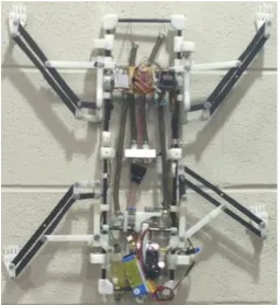
Figure 1 Proof-of-concept prototype climbing robot with onboard hydraulic system and
FAM actuators gripping a vertical wall ... 7
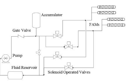
Figure 2 Hydraulic subsystem schematic ... 10
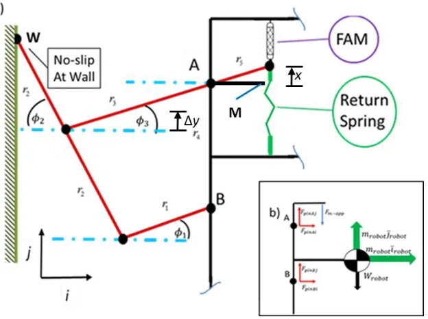
Figure 3 a) Hoeken linkage leg design schematic of upper left leg. A and B are
pin-joints connecting leg linkage to robot body, M is a mechanical stop, point W
is claw rotational joint at the wall b) Free Body diagram showing the applied
and reaction forces along with the inertial response of the robot for the upper
left quarter. ... 14
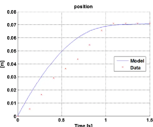
Figure 4: Experimental and model climbing robot movement during one climbing step ... 18
Figure 5: Experimental and model climbing robot current use ... 19
Figure 6: (a) Variation in robot height, (b) Muscle contraction, (c) Accumulator pressure
variance from system operating pressure, and (d) Motor speed and current with
time for three climbing steps ... 21
Figure 7: Efficiency as a function of number of steps taken by the climbing robot ... 22
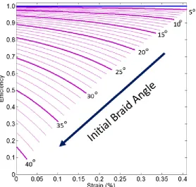
Figure 8: Efficiency as a function of contraction for initial braid angles from 5-40
degrees for ideal muscle model (blue) and non-ideal muscle model (magenta).
Curves for non-ideal model results end at the free-strain limit of the given
initial braid angle. ... 24
Figure 9: (a) efficiency and (b) velocity as a function of initial braid angle for mass
ranging from 1-5 kg ... 24
Figure 10: (a) efficiency and (b) velocity as a function of initial braid angle for operating
xi Figure 11: (a) Efficiency and (b) Velocity as a function of initial braid angle for voltages
ranging from 5-10 V ... 27
Figure 12: Actuator efficiency as a function of strain for a variety of braid radii with both
ideal (blue) and real (magenta) muscle models ... 29
Figure 13: (a) Efficiency and (b) Velocity as functions of initial braid radius and robot
masses from 1-5 kg ... 29
Figure 14: (a) Efficiency and (b) Velocity as functions of initial braid radius pressures from
500-1000 kPa ... 31
Figure 15: (a) Efficiency and (b) Velocity as a function of initial braid radius for applied
voltages from 5-10 V ... 32
Figure 16: (a) Efficiency and (b) Velocity as functions of Pump Displacement for robot
masses from 1-5 kg ... 33
Figure 17: (a) Efficiency and (b) Velocity as functions of Pump Displacement for operating
pressures from 500-1000 kPa... 34
Figure 18: (a) Efficiency and (b) Velocity as functions of Pump Displacement for applied
voltages from 5-10 V ... 35
Figure 19: Efficiency as a function of initial braid radius and initial braid angle for robot
masses of 1, 3, and 5 kg and system operating pressures of 500 and 750 kPa ... 36
Figure 20: Hydraulic system of a) SEMU and b) PVR bundle, and constant force and
actuation setup of c) SEMU and d) PVR bundle. ... 44
Figure 21: Model and experimental data for a PVR bundle consisting of a LTPMU (green)
xii and below lag pressure, and c) both pressurized at lag pressure, and d) both
pressurized and above lag pressure ... 46
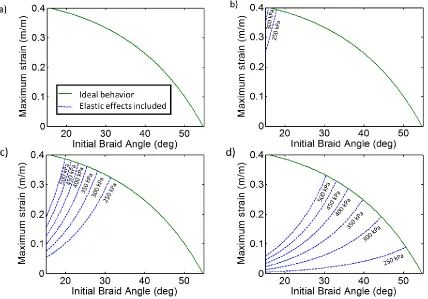
Figure 22: Relationship between initial braid angle and free strain for a) 0.5 mm, b) 1 mm,
c) 2mm, and d) 3 mm bladder wall thickness for a 6 mm radius FAM for source
pressures of 250 kPa to 500kPa. Note that as bladder thickness increases, there
is a corresponding increase in the domination of the elastic effects in limiting
the free strain... 48
Figure 23: Ideal (green) and non-ideal (blue, dashed) free strain as a function of braid angle
at 450 kPa for a 6mm radius FAM with bladders of wall thickness 2mm and 3
mm ... 49
Figure 24: Blocked force as a function of braid angle for a FAM with 6mm initial braid
radius and various bladder thicknesses at a source pressure of 450 kPa ... 50
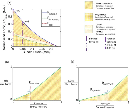
Figure 25: a) PVR bundle normalized force and strain for applied pressure of Psource,
Pth,HTPM, and Plag. Normalized force as a function normalized applied
pressure at b) zero bundle strain (blocked force condition) and c) 0.05 bundle
strain. ... 52
Figure 26: Actuator efficiency for the force and stroke characteristics of a) a PVR bundle
with two muscles and b) a SEMU with a peak pressure of 450 kPa. These plots
show the equal blocked force and free stroke, as defined. Note the area of
decreased efficiency in the PVR bundle corresponding to the area between Pth,
HTPMU and Plag and the area of increased efficiency in the PVR bundle
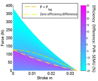
xiii Figure 27: Efficiency difference between PVR Bundle and SEMU. At pressures below
Pth,HTPM the PVR is more efficient because the HTPMU is not consuming
fluid volume. Of interest is that the percent difference is zero at Pth,HTPM ... 55
Figure 28: Force output of PVR bundle when applied pressure is source pressure, HTPMU threshold pressure, and lag pressure. ... 56
Figure 29: Applied pressure and volume consumed by the PVR bundle and SEMU for a) load 1, b) load 2, and c) load 3. Note that the maximum displacement is smaller as load increases. At high loads, the SEMU always consumes less working fluid because the HTPMU is always engaged and that at light loads and small displacements the PVR bundle always consumes less working fluid ... 57
Figure 30: 5 cycle operation performed at a constant (low) load and varying displacement. ... 60
Figure 31: 5 cycle operation at constant (low) displacement and varying load... 61
Figure 32: Load and displacement selection points for the trials shown in Table 7. ... 61
Figure 33: Operating efficiencies for varying percentages at a higher load or displacement cases ... 63
Figure 34: Actuator arrangement for a) SEMU, and b) AVR bundle ... 66
Figure 35: Normalized output force vs Actuator Strain for SEMU and AVR Bundle. ... 68
Figure 36: Hydraulic flow diagram for a) SEMU and b) AVR. ... 69
Figure 37: Electrohydraulic system diagram for continuous pump operation ... 73
Figure 38: System response to prescribed path with frequency = 0.25 Hz, xmax = 0.018 m, and mg/Fbl = 0.24 for SEMU with continuous pump operation ... 74
xiv Figure 40: Electrohydraulic system diagram for Intermittent pump operation ... 76
Figure 41: System response for a prescribed path with intermittent pump operation for
a SEMU. ... 77
Figure 42: System response for a prescribed path with intermittent pump operation for
an AVR bundle. ... 78
Figure 43: System bandwidth limits and operating region explanations for mg/Fbl = 0.24 ... 81
Figure 44: Steady-state analytical solution overlaid with dynamic simulation results for
mg/Fbl = 0.24 ... 82
Figure 45: SEMU and AVR Bundle operating limits for mg/Fbl = 0.24 ... 83
Figure 46: a) Maximum bandwidth and, b) system cycle efficiency for a variety of pump
displacements for three strains and a representative load of mg/Fbl=0.24 ... 84 Figure 47: Efficiency and bandwidth plot for a SEMU with continuous pump operation and
a load of mg/Fbl = 0.24 ... 86
Figure 48: Efficiency and bandwidth plot for an AVR bundle with continuous pump
operation and a load of mf/Fbl = 0.24 ... 86
Figure 49: Efficiency and bandwidth plot for a SEMU with intermittent pump operation
and a load of mg/Fbl = 0.24 ... 87
Figure 50: Efficiency and bandwidth plot for an AVR bundle with intermittent pump
operation and a load of mg/Fbl = 0.24 ... 88
Figure 51: Bandwidth and efficiency dynamic simulation results for a load of mg/Fbl=0.54
for a) SEMU and b) AVR bundle with continuous pump operation, and c)
xv Figure 52: Bandwidth and efficiency dynamic simulation results for a load of mg/Fbl=0.035
for a) SEMU and b) AVR bundle with continuous pump operation, and c)
1
CHAPTER I
Introduction a) FAM background and historyFluidic Artificial Muscles (FAMs) have received a great deal of attention in recent studies. Their existence dates to the 1950’s when Joseph McKibben was inspired to give increased
mobility to his daughter, who had been paralyzed by polio, and developed a ‘muscle’ actuated by
compressed carbon dioxide [1], [2]. McKibben’s original muscle and custom built control valve system included only a ‘pressurized’ and a ‘vent’ control scheme but was effective in allowing
patients to accomplish small tasks, like holding a pen, despite their paralysis. FAM’s are
biologically inspired and bear many similarities to mammalian muscles; they are single acting
and require antagonistic pairing to induce bi-directionality in force application. They respond to
external activation (i.e. fluid pressure) by producing radial expansion and axial contraction and
are capable of generating a wide variance of force profiles depending upon the loading, activation
pressure applied, and specific construction.
Recent studies experimentally characterized FAM contraction behavior and showed that
FAM force-strain production can be likened to variable stiffness springs [3]. Meller, et al. and
Tondu expanded upon this theory with analytic models and generated improved force-strain
relationships by including experimentally derived correction factors for maximum strain, blocked
force, friction, and elastic correction models [2],[4]. Bryant, et al. performed studies on the
efficiency and actuation force of variably recruited FAM ‘bundles’ and showed that more uniform
and higher efficiencies could be induced by utilizing FAMs of various sizes aligned in parallel
groups and only actuating the muscles needed for a specific force-strain regime [5]. Robinson, et
2 study on selecting the number of pneumatic FAMs which would deliver the highest efficiency for
various loading scenarios [6]. Meller, et al. and Tiwari, et al. demonstrated both the feasibility of using hydraulic FAMs rather than the traditionally used pneumatic FAMs and compared them in
force output and efficiency to similarly sized pneumatic FAMs and traditional hydraulic pistons.
Their results support the large force-to-weight ratio and efficiency advantage that hydraulic FAMs
have over the traditional hydraulic piston [7],[4], especially when grouped as bundles, enabling a
wider range of use within the force-strain space.
b) Research Aims.
This work is separated into 3 main sections which each address a previously unconsidered
area of fluidic artificial muscle research. Chapter II explores a system-level analysis of a climbing
robot which utilizes single-acting FAMs and explores the effect of various design parameters on
the total system efficiency. Chapter III uses a thin-walled elastic bladder model to explore the
feasibility of using FAM elastic nonlinearities as part of a simplified control methodology
inspired by mammalian muscle orderly recruitment. Lastly, chapter IV compares recruitment
methodologies, and electrohydraulic operating strategies to determine how they dictate the
efficiency and function of the electro-hydraulic system used to provide the motive force of
actuation.
c) Idealized FAM modeling
Idealized FAM models begin by considering the virtual work model and setting
PdV =Fdx (1)
3 Tondu, et al. [2] and others and yields a relationship between axial contraction, radial expansion,
and the angle of the braid fibers from the longitudinal axis. This geometric relationship is
developed as 0 0 cos cos L L = , and (2) 0 0 sin sin R R = (3)
where L and R are the length and braid radius of the muscle, α is the braid angle of the braided sheath, and their initial values from construction are designated as L0, R0, and α0. By performing a series of trigonometric substitutions for the volume of a cylinder, the volume of a
muscle, Vm, in terms only of strain, ε, and initial construction characteristics is shown to be
(
) (
)
3 20 0
2
0 0 2
1 1 cos
sin m
V L R
− − −
= (4)
The change in volume during contraction with respect to a change strain is shown to be
(
)
2 20 2
0
0
2 1 3 1 cos
sin m
o
d dV
L R
−
= + − (5)
Further substitution and defining strain as 0 x L
=
, where x is the change in length of the FAM and (also referred to as stroke) yields an idealized individual muscle force model of
2 2
, 0
0
1 m ideal app
x
F P R a b
L
= − −
(6)
where Pappis applied pressure and
4
2 0
1
b
sin
=
.
(8)
This idealized model is effective at predicting blocked force, especially at higher
pressures, but is generally poor at predicting free strain. Each chapter following will explore
different FAM models—chapter II uses an empirical model with predictive modification
calculating braid frication, chapters III and IV apply a predictive elastic-nonlinearity model for
5
CHAPTER II
Fully Coupled Electrohydraulic Model of a Climbing Robot: The Effect of FAM Design Parameters on System Operation (Published (2017) in Bioinspiration and Biomimetics) a) Climbing robot background
In order to gain a system-level understanding of FAMs and their interaction with the
electrohydraulic pressure generation system, a biologically inspired, four legged, FAM-actuated
climbing robot is considered. Climbing robots are testing-ground platforms for new technologies
in actuation, gait control, foot adhesion, and efficiency analysis. Actuator studies have been
performed in robots of various sizes. Large-scale climbing robots like NINJA and NINJA II
demonstrated the feasibility and effectiveness of high-powered hydraulic actuators—requiring
tethers to ensure continuity of power and required precision hydraulic alignments during
construction [8]. DC motor actuators have been effective on smaller climbing robots like ROCR
[9], which has limited payload capability. Smaller still, the gecko inspired robots, Rigid Gecko Robot (RGR) also uses DC Servo-motors while its counterpart, the Compliant Gecko Robot (CGR)
uses shape memory alloys as actuators [10]. Other climbing robot studies focus on gait analysis
and locomotion methods rather than system efficiency and longevity of operation [11]. Climbot, for example, makes use of a variable degree of freedom gate strategy analyses with antagonistic pairing of “rubbertuators” to enact a non-planar gait in an inspection robot. Robug focuses on the
control-algorithm driving its gait and foot-adhesion techniques with its pneumatic legs [12, 13].
Still other climbing robots focus almost exclusively on foot-adhesion techniques: the CLIBO
design uses a 4 DOF DC-motor-driven robot for analysis of a gripping method toward maintaining
a stable position for a prolonged period [14]. These climbing robots have been at the forefront of
6 DC motor robotic actuators are at a disadvantage when compared to FAMs due to increased
weight, alignment criteria, and large variations in electrical power consumption during operation
[2]. Furthermore, hydraulic piston-cylinder assemblies are heavier per force output than FAMs,
sensitive to alignment, and make use of sliding seals which are prone to leak or degradation [7].
In addition to their high force output and light weight construction, FAMs also offer a smooth,
naturalistic motion that is well suited to bio-inspired legged robot architectures.
Previous studies have focused on the operation, control, and efficiency of the FAMs
individually, in groups, and even in antagonistic pairs, but in isolation from the system which
generates the pressure utilized by the muscles [15]. The purpose of this study is to determine how various FAM and system components affect the efficiency and effectiveness of the system’s
operation. It will do so by generating a fully coupled electro-hydraulic model of a climbing robot
with FAM actuators, validating this model against data from a climbing robot of like-design, and
using the model to study the effect of design and operating parameters on system efficiency and
velocity of the robot.
b) System Overview
A simple, bio-inspired climbing robot is considered. In this robot concept, a DC motor
operating with a prescribed applied voltage drives a constant volume positive displacement pump
to form the hydraulic power source. The pump pressurizes a gas-charged accumulator which is
connected to a network of valves directing fluid to the artificial muscle actuators. The FAMs are
used as linear tensile actuators to drive the limbs of the robot. Each limb and FAM actuator pair
is assumed to have identical parameters, including a kinematic relationship described in section
7 figure 2 and is discussed in section 2.2. A complete description of the proof-of-concept climbing
robot, its construction, and hardware components can be found in Bryant, et al.[16].
Figure 1: Proof-of-concept prototype climbing robot with onboard hydraulic system and FAM actuators
gripping a vertical wall.
The FAMs provide single acting tensile actuation and therefore a linear return spring is
included to extend the muscle and leg during depressurization. The robot performs climbing
locomotion by making use of claws, which are modeled as a no-slip condition on the vertical wall.
During climbing the appropriate FAMs are inflated with working fluid from the accumulator.
The actuators then contract, moving the robot vertically while the un-activated muscles are vented
and allowed to extend from the force applied by the return springs. In order to fully understand
the electrohydraulic coupling to the mechanical operation of the climbing robot, this study begins
8 is followed by an analysis of the pump-motor combination and a dynamic model of the motion of
the robot itself.
i. FAM subsystem
First, an accurate model of FAM force-contraction behavior is applied to the system under study.
The most basic fluidic artificial muscle models were discussed previously and ignore losses and
assume constant surface area and a during bladder inflation while maintaining a cylindrical shape.
Later studies have generated correction-factors which address energetic losses in the form of
friction, elasticity, and non-cylindrical shape near the tips of the muscle. The model employed
here includes empirically-determined correction factors to address these construction-associated
losses. We express the muscle force-contraction model in terms of the contraction, x, rather than
the more typical nondimensional strain,
, by making the substitution,0 x l
= where lo is the
initial muscle length. The key performance-driving parameters of fluidic artificial muscles are
the initial braid angle, αo, initial braid radius, ro, and applied pressure by the working fluid, Papp. FAM output force, Fm initially proposed by Tondu [17] and is fully developed and tested by Meller, et al. [4] as
2 2
0
0 1
m app F
x
F P r a b
l = − − (9)
( )
2 ,(
)
0meas max F
app F
r P a b
=
− (10)
( )
, 0
1 1 1 3 cos meas max = −
(11)
9 strain for a given pressure application. These correction factors are determined for a specific
muscle and act to correct differences between calculated and observed force characteristics,
largely from inherent elastic bladder effects in the FAM contraction. In this study, the correction
factors were determined for the muscles from the experimental climbing robot at system pressure
and have values shown in table 3. The model is predicated on the assumption that FAMs retain
an approximately cylindrical shape during their quasi-static contraction, and the correction factors
help correct for the portions near the tips of the FAMs which do not maintain that shape.
Tondu expanded upon his original modeling by generating a braid on braid frictional
force, which accounts for both static and kinetic friction [17]. This frictional force is represented as
( )(1/ )
(
( ))
fric con app
F
=
f
S
P
sgn x
(12)where x is muscle contraction rate, and f is the total dry friction coefficient and is determined
by
/
(
)
x xsk s k
f
=
f
+
f
−
f e
− (13)with fs and fkbeing the static and kinetic friction coefficients of the braid material,xsis a
material based velocity constant, and 1/ is the estimated ratio of the muscle’s lateral self-surface
contact. Sconis the braid-to-braid surface area of contact, and is defined as [17]
(
)
sin 12
2 1 2
1 cos 1
o
S r l
con o o x
10 We combine the force and strain correction factors with the frictional loading parameters in order
to capture both bladder elasticity and friction effects, yielding an output force model which takes
into account the primary loss criteria for FAMs.
ii. Hydraulic subsystem
Figure 2: Hydraulic subsystem schematic.
Upon modeling of the FAM contraction characteristics, it is next necessary to couple this
contraction with the hydraulic-actuation power-source. The hydraulic system considered is
shown in figure 2. The system diagram shows four muscles grouped into two pairs; each muscle actuates a single leg on the climbing robot with two legs moving simultaneously for each step.
The working fluid analyzed is water due to its relative incompressibility and its compatibility with
the system components. A series of equations describing the fluid flow through the system are
11 contraction are of foremost importance. The fluid volume consumption as a function of length
by an actuated FAM, Vm, is developed by Tondu as
3
0 0
2
0 0 2 2
0 0 1 1 1 sin tan m x x l l
V r l
− − = − − (15)
The chain rule is utilized on equation (9) to determine the time rate of change of the
volume consumption,Vm as
2
0 0 0
2
0 0 2 2
0 0 1 1 3 1 sin tan m x
l l l
V r l x
− − = + (16)
where xis the time rate of contraction. In order to determine the pressure drop in the accumulator due to muscle contraction, we relate the gas volume change in the gas-charged accumulator to the
volume consumed by the muscles and the fluid added by the positive displacement pump, yielding
, , ,
acc initial acc initial acc
acc initial m p
P V
P
V V V
=
+ − (17)
by use of the ideal gas law with a constant temperature approximation, where Pacc is accumulator pressure and Vp is the volume added to the accumulator by the pump. There is a conditionally opened bypass valve which maintains operating pressure at or below initial system operating
pressure. The pressure transmitted by the accumulator to the muscle is similarly derived using
first principles, resulting in
2 2
, 2
m p m
app acc l
acc m inlet
V V V
P P h
12 where Vp is pump flowrate, Am,inlet is the cross sectional areas of the muscle inlet— defined to be
the initial cross sectional area of the FAM, and Aacc is the cross sectional area of the accumulator. Pipe losses are modeled as
, 2 2 fl m m inlet L V A h k g = (19)
where kfl is the pipe fluid friction coefficient, based on a combination of the fittings and piping used and result in less than a 1% loss in pressure from the accumulator to applied to the muscle.
iii. Electrical subsystem
The hydraulic system pressure is created and maintained by a constant-volume positive
displacement pump with displacement, D, This pump is driven by a brushed DC-motor with an applied voltage. The hydraulic pump and motor assembly used on the proof-of-concept robot are
an off the shelf HP-48030 hydraulic pump and DC motor from HP-Tech [18]. Based on first principles of torque balance and making use of Kirchoff’s Voltage Law, the motor-pump
rotational acceleration, , is modeled as
e m p fric
k I B J
= − − − (20)
where fricis motor friction, J is the motor’s moment of inertia, k
eis motor’s torque constant, and
Bmisfrictional damping coefficient. The rate of change of current, I , can be shown to be
motor b
V k IR
I
L − −
= (21)
where kb is back electro-magnetic force constant, L is motor inductance [19], and motor-pump
13
2
acc p
P D
=
.
(22)
As shown in table 1, current and motor speed are set to be initially zero (open circuit) and allowed
to adjust as required to meet the other system inputs after a switch is closed at t=0. Table 1. Initial conditions of key
electrical parameters
Parameter
(units)
Initial Value
I(A) 0
(rad/s) 0
iv. Climbing dynamics
A Hoeken-linkage leg mechanism is selected for the study due to its ability to translate
rotational movement about a revolute joint into linear motion of the end effector, allowing for a
linear climbing stroke with a single degree of freedom at each leg [20] . The robot is moved by
four Hoeken-linkage legs operated in pairs and assuming negligible leg mass compared to the
14 Figure 3: a) Hoeken linkage leg design schematic of upper left leg. A and B are pin-joints connecting leg linkage
to robot body, M is a mechanical stop, point W is claw rotational joint at the wall b) Free Body diagram showing
the applied and reaction forces along with the inertial response of the robot for the upper left quarter.
Figure 3 shows the leg mechanism, including FAM and return spring connections along
with relevant kinematic labels. In order to avoid nomenclature conflicts during the climbing
movement analysis, movement along the horizontal axis is labeled in figure 3 as i and movement along the vertical axis is similarly labeled as j. Linkages r1-r5 were selected to have lengths such
that linearity was optimized [16, 20] and angles
1-3 change based on the contraction of the FAM. We relate muscle contraction, x, to the robot body by5 3
r sin
x=
. (23)The position of the robot, y, measured at point A relative to the no-slip condition assumed at the claw-to-wall connection point, W, is
3 3 2 2
r sin sin
15 Since the system has a single degree of freedom, performing a loop closure analysis allows the
use of
2 2 2 2
1 3 2 r4 23 2(sin 3sin 2 3cos 2) 23 4sin 3 22 4r sin 2
r =r + + +r rr −cos − rr − r (25)
to relate
2 to
3. At the beginning of each step, link r3is horizontal and angle 3is zero. The applied muscle force to the system acts vertically and is calculated asm app m spring fric
F − =F −F −F +T (26)
where tension, T, represents the force from a mechanical stop that prevents upward leg extension
beyond the
3 =0position. It is defined such that when Fm−Fspring −Ffric =0, mrobotjrobot =0.It ensures that mathematically, FAM length never extends beyond lo and allows the robot to maintain static equilibrium even when applied pressure is zero. The spring is a linear
return-spring and has a force of Fspring=0 at x=0. The return spring is never compressed, and the value
of x is never negative. In order to relate the applied end-effector forces to the rotational torque about point W, we use the Jacobian analysis of the linkage system [19], defined as
2 3 2 3 A A W A A A i i J j j − = (27)
where JW A− is the Jacobian relating translational motion of the pin-joint at point A to the rotational
motion about the joint robot’s claw at W.
2
A i
is the partial derivative of the horizontal motion of
point A with respect to
2, while2
A j
16 with respect to
2. While the movement of point A is dependent on
3 as well as
2, by equation (19), we have
3 = f( )
2 and, therefore equation (21) can be expressed as2 2 A W A A i J j − = (28) W B
J − is similarly constructed for pin-joint B and JW M− for the point of muscle attachment. We
apply the virtual work [19] model for Jacobian analysis to show that
T W A JW AFpinA
− = − (29)
where
W A− is the torque about the wall-joint at the robot claw induced from the pin-reaction force, TW A
J − is the transpose of the Jacobian from pin A to the wall joint, and FpinAj is the vertical pin
reaction force at point A. This process is repeated using the vertical force at the other leg-body
pin joint, FpinBjto find
W B− , applied muscle force, Fm-app to find
W M− , andW
robotto find
W R− , the torque from the robot’s weight at its center of gravity. The equations of motion of the robotcan be written as
2
W W A W B W M W R
I
=
−+
−+
− + − (30)) )
( pinAi pinBi L ( pinAi pinBi R
robot robot
m i = F +F + F +F (31)
and mrobot robotj =FpinAj+FpinBj−Fm app− −Wrobot (32)
where IW is the time-varying moment of inertia of the robot’s center of gravity about point W, and
horizontal acceleration of the robot,
i
robot, is zero based on the restrictions of the Hoeken linkageassembly, and
(
F
pinAi+
F
pinBi)L R/ is the horizontal pin reaction forces from the leg on each side17 formulae give the relationships governing the motion of the robot in terms of muscle force
generation as a function of contraction and applied pressure. Initial conditions for this subsystem
are shown in table 2.
Table 2. Initial conditions of key climbing subsystem parameters Parameter
(units)
Initial Value
x(m) 0
3
(rad) 0
spring
F (N) 0 (x=0)
j (m) 0
c) Model Validation
The model output is compared to results measured from the climbing robot shown in
figure 1. The parameter values for this prototype robot are listed in Table 3. These parameters
were directly measured, or, in the case of the motor-pump assembly, provided by the component
manufacturer. The experimental results are collected using 2D video motion analysts to measure
the position of the robot as a function of time and an onboard ammeter and data logging to record
current [16]. Comparison of both operating current and robot motion were found using the system
of coupled equations previously listed. Model operating current and robot motion as functions of
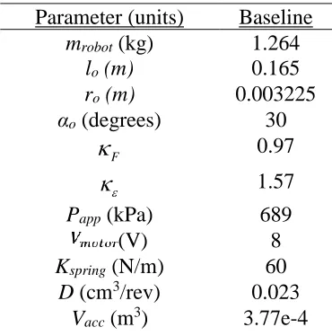
time were found using the system of coupled equations previously defined. Table 3. Initial parametric values
Parameter (units) Baseline
mrobot (kg) 1.264
lo (m) 0.165
ro (m) 0.003225
αo(degrees) 30
F
0.97
1.57
Papp(kPa) 689
(V) 8
Kspring(N/m) 60
D (cm3/rev) 0.023
18 Table 3 (Continued). Initial parametric
values
No-load speed (RPM) 17000
No-Load Current (A) 0.5
𝑘f 𝑘e
𝑘𝑏
(Nm/A) 17.1e-3
𝑘e (V.sec/radian) 17.1e-3
Bm (Nm/(rad/s)) 1.23e-6
J (kg.m2) 9.45e-7
R (Ohms) 0.45
L (H) 0.112e-3
Vacc,I(%) 50
Figure 4: Experimental and model climbing robot movement during one climbing step.
Figure 4 plots the vertical position of the robot during one climbing step (i.e. a single
contraction of a leg pair), and shows that the model predicts the positon at the end of the step to
within 1.1% of the measured value. This is vitally important to the usability of the model, since the primary measure of the system’s energy output is the change in potential energy after a
specific number of total steps. The apparent mismatch between the model and the data during
this contraction is due to the model-assumed instantaneous valve-opening which allows
instantaneous flow into the FAM. Since real valves take some time period to open and allow
19 perfectly aligned, the average velocity between time t = 0.2 seconds and time t = 0.8 seconds
matches to within 1.5%. The initial and final leg positions are the primary drivers of system
output and therefore, the match of 1.1% as seen in figure 4 is sufficient for our analyses. Figure
5 shows a clear overlap of experimental and predicted current draw throughout motor starting
operation; the initial current spike, and final steady state operating currents are of particular note.
The model is therefore satisfactorily accurate in its prediction of system current draw over time.
Figure 5: Experimental and model climbing robot current use.
These validation tests demonstrate that the model reasonably captures the mechanical and
electrical behavior of a physical meso-hydraulic climbing robot with FAM actuation. It can
therefore be used to perform case studies for the purpose of understanding the dependencies of
system-level performance metrics like locomotion speed and efficiency on the design and
operating parameters of the robot.
d) Simulation of Continuous Climbing Operation
Next, the model is used to analyze the response of the system during continuous climbing.
The simulation is started with a zero current condition and is initialized at rest. The system
parameter values are set as shown in Table 3. Applied voltage and muscle contraction are enacted
20 that the next step can be performed. The simulation is set to have the robot perform a
predetermined number of steps by alternating actuation of leg pairs. The top right and bottom
left legs are actuated together as leg pair 1 and the top left and bottom right legs are actuated as
leg pair 2. We define system efficiency as the ratio of output work to input energy for the climbing
locomotion. Considering locomotion to start from rest and end at rest, the system efficiency is
given by
Δ robot
sys
motor U
P dt
=
(33)where instantaneous power input, Pmotor is calculated as the constant operating voltage multiplied
by the instantaneous motor current, and ΔUrobot is the change in robot gravitational potential
energy following a climbing operation.
The output results for the climbing robot model parameters performing a 3-step climbing
sequence are shown in figure 6. As muscle contraction occurs, fluid volume is consumed from
the accumulator, resulting in a pressure drop in the accumulator, thereby inducing a motor torque
decrease and speed increase. As the pump operates to re-pressurize the accumulator to the
prescribed operating pressure, torque increases and motor-speed drops. This speed change
directly affects operating current, and therefore power consumption. There is an initial current
spike correlating to the startup of the motor; this is followed by smaller current fluctuations during
the climbing gait cycle. The position dwells at each step occur due to the mechanical range of
21 Figure 6: (a) Variation in robot height, (b) Muscle contraction, (c) Accumulator pressure variance from system
operating pressure, and (d) Motor speed and current with time for three climbing steps.
After the initial starting current spike, the system operates at a near constant current draw,
yielding an improved system efficiency as the duration of operation increases. Figure 7 shows
efficiency as a function of the number of steps taken. As the number of steps increases, the
starting current of the motor makes up a smaller percentage of the overall energy usage while the
output work remains constant per step. This represents an interesting potential advantage of this
electrohydraulic actuation scheme for a legged robot. In a more conventional approach using a
servomotor at each leg DOF, a starting current spike would be encountered at each step. The
hydraulic power system used here, however, allows the single motor to run continuously and
distribute power among the legs. The peak efficiency seen for a long operational period of this
22 which follow will bring to light design characteristics which can altered in order to improve this
peak efficiency.
Figure 7: Efficiency as a function of number of steps taken by the climbing robot.
e) Parameter Sensitivity Studies
... The model is next used to study the effects of various parameters on the
electro-hydraulic system performance as defined by average robot velocity and system efficiency.
Parameters to be investigated are categorized as either design parameters: pump displacement, initial braid angle, and initial braid radius, or operating parameters: robot mass, system voltage, and system operating pressure. Values not being varied in a given study were fixed at the
values for the baseline climbing robot as shown in Table 3. The parametric sensitivity study is
performed by simulating the system across a sweep of design parameter values for several
operating parameter cases to reveal the interdependencies of the system configuration
i. Investigation of initial braid angle sensitivity
As a key actuator design characteristic, initial braid angle is swept from 25-40 degrees to
23 these various initial braid angles first to find if there is any deviation between traditional
actuator-focused FAM research and the system-level approach performed here.
1) Sensitivity of actuator efficiency to initial braid angle
An actuator-only quasi-static analysis of an idealized FAM (no friction,
F=1,
=1) and a real model which includes the empirically-determined frictional losses and correction factors isperformed to determine the effect of initial braid angle on the actuator efficiency. Actuator
efficiency is defined as
m act
F dx
PdV
=
(34)
where
actis the actuator efficiency, Fm is the muscle force and P is the fluid pressure applied to the muscle. The results, as shown in figure 8, indicate that while an idealized muscle is 100%efficient with any initial braid angle, as initial braid angle increases in a non-ideal FAM, there is
a correlating negative effect on both maximum achievable strain and actuator efficiency. These
strain and efficiency limitations in comparison to an idealized model are consistent with the
24 Figure 8: Efficiency as a function of contraction for initial braid angles from 5-40 degrees for ideal muscle model
(blue) and non-ideal muscle model (magenta). Curves for non-ideal model results end at the free-strain limit of the
given initial braid angle.
2) Effects of robot mass and initial braid angle on system performance
25 Figure 9 illustrates the significant effect initial braid angle has on both system efficiency
and robot velocity. Figure 9(a) shows a distinct peak efficiency value and its corresponding initial
braid angle for each robot mass tested. Robot mass affects both the value of this peak and the
initial braid angle at which it occurs. For a robot mass of 1kg, the peak efficiency occurs at an
initial braid angle of 32.6 degrees while for a robot mass of 5kg, the peak efficiency occurs at
29.8 degrees. As mass increases from 1-5 kg, the system’s efficiency also becomes more sensitive
to changes in initial braid angle. The increased efficiency for a heavier robot is indicative of an
over-powered FAM at a given braid angle. The rapid drop of the 5kg case to 0% efficiency when
the initial braid angle is increased to 36.2 degrees is indicative of the initial braid angle being
sufficiently large that the muscle underpowered and unable to contract under the robot load, which is predicted by equation (1). As the robot’s mass increases, its velocity at all initial braid angles
decreases. By comparing the two plots, it is noted that the initial braid angle at which peak
velocity and peak efficiency occur is the same point, yielding an important design criterion.
It is interesting to note that while lower initial braid angles increase the peak force output
of the actuator, they do not correspond to maximum system efficiency nor maximum robot
velocity. To understand this result, we must recognize that peak muscle contraction also is related
to initial braid angle. This contraction leads to an increase in volume consumption by the muscle,
as shown in equation (9), and lower initial braid angles thus consume more pressurized working
fluid. This increasedvolume consumption causes increased accumulator refill time and therefore
larger electrical power consumption and a longer cycle-rate and lower robot velocity. This
analysis underscores the importance of considering braid-angle during system design; too small
26 insufficient force output and lead to a potential for incomplete range of motion, an effect
magnified by an increase in system load.
3) Effects of operating pressure and initial braid angle on system performance
Figure 10: (a) efficiency and (b) velocity as a function of initial braid angle for operating pressures from 500-1000
kPa.
The sensitivities of system efficiency and average velocity for initial braid angles from
25-40 degrees and operating pressures from 500-1000 kPA are shown in figure 10. The results
indicate that at each pressure, there is a distinct initial braid angle for which both efficiency and
velocity are maximized. At 500 kPa, this optimal initial braid angle is 32.1 degrees and at 1000
kPa it increases to 32.8 degrees. Of interest, as with the mass analysis, is that lower braid angles
lead to increased volume consumption and decreased efficiency. Also, at higher braid angles, the
FAMs are underpowered, as predicted by equation (1), so while volume consumption is lower,
the decrease in energy output of the system—shorter leg strides—dominates the efficiency of the
system. This effect can be overcome somewhat by increasing system operating pressure as seen
in the efficiency plot overlap at approximately 36 degrees in figure 10(a), but only slightly, since
27 between 32 and 33 degrees yields the best performance over the pressure range tested and that,
furthermore, the lowest pressure which will effectively perform the motion should be selected if
maximizing efficiency rather than velocity is the goal.
4) Effects of applied voltage and initial braid angle on system performance
Figure 11: (a) Efficiency and (b) Velocity as a function of initial braid angle for voltages ranging from 5-10 V.
Initial braid angle is swept from 25-40 degrees for applied system voltages of 5-10 V. The
results, shown in figure 11, indicate that voltage has a significant effect on efficiency, but little
effect on the velocity of the system. Also, unlike both robot mass and system operating pressure,
system voltage has almost no effect on the initial braid angle at which peak efficiency occurs.
This is because voltage has no direct effect on output force or volume consumption, as indicated
in equations (1) and (9)As with both pressure and mass changes, however, the system becomes
more sensitive to initial braid angle as voltage is increased. While voltage has a significant effect
on efficiency at all initial braid angles, only at lower initial braid angles does the higher voltage
result a marginal increase in velocity—due to a lower accumulator refill time. But, as initial braid
28 Based on this information, when designing an electrohydraulic system for operating in conjunction with FAM’s, the lowest operable voltage should be selected.
ii. Investigation of initial braid radius sensitivity
Initial braid radius is another key actuator design characteristic, having an impact on force
output, surface area and frictional losses, and volume consumption. We begin with a study of the
actuator alone, and then perform a sweep of initial braid radii for analysis with mass, pressure,
and voltage.
1) Sensitivity of actuator efficiency to initial braid radius
A sweep of braid radii from small (1.5 mm) to large (6.5 mm) is performed for an ideal actuator and a non-ideal actuator as defined in section 5.1.1. The results are shown in figure 12.
For all braid radii, the ideal muscle exhibits an efficiency of 1 as defined by equation (26).
However, as braid radii decreases, both the peak strain and the peak efficiency decreases as well.
This indicates that for a given application, one would select a FAM with the largest possible braid
radius, but, as can be seen in subsequent sections, this is not the case when designing for the
29 Figure 12: Actuator efficiency as a function of strain for a variety of braid radii with both ideal (blue) and real
(magenta) muscle models.
2) Effects of robot mass and initial braid radius on system performance
Figure 13: (a) Efficiency and (b) Velocity as functions of initial braid radius and robot masses from 1-5 kg.
Initial braid radii from 2.5-5mm for a range of masses from 1-5 kg were considered to
produce the system efficiency and average velocity results shown in figure 13. For all masses,
30 because at low braid radii, output force is insufficient for complete muscle contraction—the
FAMs are underpowered and this limits the cycle rate and the energy output. Peak system
efficiency increases with mass over the entire range tested as it did in the mass-braid angle study;
this is due to the increased energy output possible with a more massive robot. The optimal braid
radius increases with increasing mass over the entire range due to the increased force output
required to move the load. Because the output force of the muscle as described in equation (1)
increases quadratically with the radius, FAMs with large radii can become overpowered—that is,
they have a higher peak force output than necessary to reach full contraction allowed for the given
load. The increased volume consumption in this case drives the system efficiency down rather
than the contraction-limitations which occur at smaller, less forceful braid radii. The peak
efficiencies and peak robot velocities occur at the same braid radius for a given mass, because
volume consumption and average step-cycle rate are linked. As shown in equation (11), the larger
volume consumed by the muscle, the more volume must be restored by the pump in order to
restore operating pressure to its initial value. This requires more time, so step-cycle speed
decreases. As mass increases at smaller braid radii, the efficiency drops due to the muscle
31
3) Effects of operating pressure and initial braid radius on system performance
Figure 14: (a) Efficiency and (b) Velocity as functions of initial braid radius pressures from 500-1000 kPa.
The same range of braid radii are considered over a range of operating pressure from
500-1000 kPa in figure 14. As with the mass-sensitivity study, changing pressure affects peak system
efficiency and the initial braid radius at which peak efficiency occurs. In increasing initial braid
radius from 2.5mm to its optimal value, the lowest pressure demonstrates the highest sensitivity
to initial braid angle. At initial braid radii greater than the optimal value, higher pressure shows
an increased sensitivity to braid radius. Increasing pressure has a positive effect on robot velocity
at lower braid radii, but this advantage decreases as braid radius increases beyond the optimal
value. The positive impact of pressure on velocity and efficiency at low braid radii is because of
the underpowered nature of the smaller FAMs. As the FAMs increase in size, the impact of the
radius in volume consumption dominates the work output. Furthermore, at low braid radii, the
lowest pressures fail to fully contract the FAM, resulting in low efficiency and velocity outputs.
As with previous analyses, the balance between ensuring sufficient FAM output force while
minimizing volume consumption is essential for achieving both optimal efficiency and robot
32
4) Effects of applied voltage and initial braid radius on system performance
Figure 15: (a) Efficiency and (b) Velocity as a function of initial braid radius for applied voltages from 5-10 V.
Braid radius is next swept through the range of 2.5-5 mm for applied voltages from 5-10
V in figure 15. As with initial braid angle, when the FAM is underpowered, as at lower braid
radii, applied voltage has no effect on the velocity of the system. While increasing voltage
negatively affects the system efficiency, it has a negligible effect on the sensitivity of efficiency
to initial radius. At all braid angles, using a higher system voltage is less efficient due to the
larger power consumption of the system with negligible decrease in operating time. We see here,
again, for an improved efficiency, the lowest usable voltage is best.
iii. Investigation of pump displacement effects
Pump displacement per revolution is an important design choice because it provides the
physical coupling between the electrical and hydraulic aspects of the system. It directly impacts
operating motor torque, pressure recovery and maintenance, and volumetric flowrate into the
accumulator. Pump displacement is swept from values of 0.01 – 0.1 cm3 for a range of robot
33 ideal pump displacement for the system in question and if so, whether and how that pump
displacement is affected by other system parameters.
1) Effects of robot mass and pump displacement on system performance
Figure 16: (a) Efficiency and (b) Velocity as functions of Pump Displacement for robot masses from 1-5 kg.
Figure 16 plots the resultant efficiency and velocity output plots as functions of pump
displacement for robot masses from 1-5 kg. For each mass, there is an ideal pump displacement
which correlates to the peak efficiency of the system as well as sharp change in the slope of the
velocity curves. This point correlates to the pump displacement at which volumetric consumption
by the FAM is more limiting than volumetric flowrate into the accumulator by the pump,
governed by equations (11), (14), (15), and (16). At lower pump displacements, the FAM has
reached contraction equilibrium prior to the accumulator being re-pressurized to its initial value.
At higher pump displacements, the accumulator is refilled quickly, so it is FAM contraction
equilibrium which drives cycle-rate. As can be seen in figure 16(b), at very low pump
displacements, the motor can operate near its peak speed but not refill the accumulator quickly,
34
2) Effects of operating pressure and pump displacement on system performance
Figure 17: (a) Efficiency and (b) Velocity as functions of Pump Displacement for operating pressures from
500-1000 kPa.
In figure 17, pressure is swept from 500-1000 kPa for the same range of pump
displacements. Increasing operating pressure increases pump torque, and therefore, system power
consumption. This results in an efficiency drop at all pump displacements considered. Pressure
has a negligible effect on the velocity of the robot in comparison to the pump displacement since,
for the mass given, even the lowest applied pressure considered is sufficient to fully contract the
FAM; therefore volume consumption is independent of pressure in the load case considered.
Since volume consumption is not changed by pressure for this robot mass, the system efficiency
is decreased from higher operating torques required for increased pressures. This indicates that the pump be designed such that the motor’s steady-state operating speed is at or near its peak
35
3) Effects of applied voltage and pump displacement on system performance
Figure 18: (a) Efficiency and (b) Velocity as functions of Pump Displacement for applied voltages from 5-10 V.
Figure 18 plots the system efficiency and velocity when voltage is varied from 5-10V for
the same range of pump displacements. As with changes in pressure and mass, the velocity of the
robot is largely unaffected by changes in applied voltage when compared to the pump
displacement sensitivity. System efficiency is more sensitive to pump displacement changes at
higher voltages, in addition to being less efficient. Increasing system voltage does increase
operating motor speed, but this speed increase results in a larger current draw, so, as with the
voltage studies performed in both FAM design studies, it is ideal to operate at the lowest
reasonable voltage for the electrical system being designed.
f) Muscle Selection Case Study and Discussion
Based on results presented in Section 5, it is apparent that, while the FAMs exhibit
improved actuator efficiency with smaller initial braid angles and larger initial braid radii, these
straightforward trends do not necessarily hold when the system-level efficiency is considered. In
order to delve deeper into the design and selection of muscle actuators for the climbing robot, a