HAN, TAE SIK. Efficient Subsequence Matching with LCS. (Under the direction of As-sistant Professor Jaewoo Kang.)
Advances in sensors and wireless network technologies have produced many sensor net-work applications. In a typical setting, a large number of different types of sensors are deployed over a wide area. The sensor streams generated from individual sensors are then combined in a server node, naturally forming a multivariable time series, and then saved in a storage system. Searching and mining interesting patterns from this multivariable time series dataset is a key challenge in time series analysis.
divided into a series of disjoint equi-length subsequences which are then indexed in an R-tree. We introduced a new way to compute the similarity bound in the index matching framework using LCS. The proposed query matching scheme that is named as multiple window sliding scheme, reduces many false alarms encountered in the previous approaches. We also developed an algorithm to skip expensiveLCScomputations by observing the warping paths.
by
Tae Sik Han
A dissertation submitted to the Graduate Faculty of North Carolina State University
in partial fulfillment of the requirements for the Degree of
Doctor of Philosophy
Computer Science
Raleigh, North Carolina 2007
Approved By:
Dr. Xiaosong Ma Dr. Ting Yu
Dr. Jaewoo Kang Dr. Rada Y. Chirkova
DEDICATION
To the past of my parents, my parents-in-law, and my wife, Hee Jin, for their sacrifice and support.
BIOGRAPHY
ACKNOWLEDGEMENTS
Foremost, I would like to thank my advisor, Dr. Jaewoo Kang, for his thoughtful direction and affectionate encouragement. This dissertation would not have materialized without his careful guidance and continuous support. I owe Dr. Kang every bit of credit for my research accomplishments and exciting experiences I encountered during my doctoral work at NCSU. I would like to acknowledge my advisory committee members, Drs. Rada Y. Chirkova, Xiaosong Ma, and Ting Yu for their enlightened comments and constructive suggestions related to my work.
I also would like to thank Dr. Seung-Kyu Ko for his valuable comments and advice on my dissertation work. The IT national scholarship program of the Korean Government that partially supported my graduate study is gratefully acknowledged. The last two years of study at NCSU were supported by the North Carolina Office of State Auditor and the SAS Institute. I sincerely appreciate their support which enabled the accomplishments presented in this dis-sertation. I would like to thank Dr. Eamonn Keogh for his papers and datasets that were very useful in experiments to validate idea. I would like to thank Dr. Lennox Superville for giving me a chance to join his project and for his invaluable advice to keep concentrating on my Ph.D. work. I would like to thank my direct manager, Craig Rubendall, at SAS for being my mentor and for placing his trust in me.I would like to thank Ms. Vilma Berg for her proofreading and advice in the final stage.
Contents
List of Figures ix
List of Tables xi
1 Introduction 1
2 Background and Related Work 9
2.1 Notational Conventions . . . 9
2.2 Subsequence Matching Framework (Dual Match vs. FRM) . . . 10
2.3 Dual Match Subsequence Matching with Euclidean Distance . . . 11
2.4 Non-Euclidean DistanceDTW andLCS . . . 12
2.5 Optimal Bounding for Index Matching . . . 16
2.6 Sequence Alignment . . . 17
2.7 Other Related Work . . . 18
3 Subsequence Matching withLCSUsing Dual Match Index in Single Channel 19 3.1 Problem Statement . . . 19
3.2 Linear Search and SkippingLCSComputation . . . 21
3.2.1 Alignment inLCS . . . 22
3.2.2 SkippingLCSComputation . . . 22
3.3 Indexing . . . 24
3.4 Index Matching withLCS . . . 24
3.5 Window Sliding Schemes in Index Matching . . . 25
3.5.1 Simple Single Window Sliding . . . 25
3.5.2 Single Window Sliding . . . 27
3.5.3 Multiple Window Sliding . . . 28
3.6 Post-Processing and Skipping . . . 30
3.6.1 Post-Processing . . . 30
3.6.2 Skipping theLCSComputation . . . 31
3.7.1 Different Sliding Schemes and Candidates . . . 32
3.7.2 Goodness and Tightness . . . 37
3.7.3 Improving Performance by Skipping Similarity Computations . . . 37
3.7.4 Runtime . . . 39
4 Multivariable Subsequence Matching 42 4.1 Introduction . . . 42
4.2 Notational Conventions . . . 46
4.3 Problem Statement . . . 48
4.4 Indexing for Multivariable Time Series . . . 49
4.5 Index Matching in Multivariable Time Series . . . 50
4.6 Post-processing . . . 52
4.7 Skipping withLCSfor Multivariable Time Series . . . 52
4.8 Experiment of Multivariable Time Series Dataset . . . 53
4.8.1 Different Sliding Schemes and Candidates in Multivariable Time Se-ries Data . . . 53
4.8.2 Goodness and Tightness . . . 59
4.9 Improving Performance by Skipping Similarity Computations . . . 59
5 Conclusion 62
6 Appendix: First 500 Points of Datasets 64
List of Figures
1.1 Sleep Apnea: An Example of Time Series Analysis [1], wk :wake, slp:sleep . . 2
1.2 Whole Sequence Matching in a Single Channel . . . 4
1.3 Subsequence Matching in a Single Channel . . . 5
1.4 Subsequence Matching in a Multivariable Data . . . 6
2.1 Two Subsequence Matching Frameworks . . . 10
2.2 An Example ofDTW Computation . . . 13
2.3 An Example ofLCSComputation . . . 15
2.4 Euclidean,DTWandLCSWhen Noise Involved . . . 16
3.1 Matching Subsequences in Subsequence Matching . . . 20
3.2 Alignment withLCSwhen|Query|= 32 and|Data|= 48 . . . 21
3.3 An Example of SkippingLCSComputation when|Q|= 4 andδ= 1 . . . 23
3.4 Indexing and Index Matching wherew=9 andN=3 . . . 25
3.5 Window Sliding Schemes when|v|=4. . . 26
3.6 Matching points (connected by dotted lines) are not captured in the index matching usingLCS . . . 26
3.7 Index Matching Result . . . 29
3.8 Postprocessing determines the entire lengths of the candidate subsequences . . 31
3.9 Candidate Ratio = # of candidates by multiple windows sliding# of candidates by single windows sliding . The same color indicates queries of the same length. . . 33
3.10 Summary of Candidate Ratio in Figure 3.9 . . . 34
3.11 Index . . . 35
3.12 Goodness and Tightness . . . 36
3.13 Skipping Similarity Computations . . . 38
3.14 CPU Time for FRM, Single Window Sliding and Multiple Window Sliding Scheme . . . 40
4.1 Multivariable Subsequence Matching . . . 43
4.2 Windows, Frames and Channels in a Multivariable Time Series . . . 47
4.3 An Example of an Index that ShowsMBRsand Windows . . . 49
4.4 An Example of Multivariable Subsequence Matching . . . 51
4.5 Candidates Ratio= # of candidates by multiple windows sliding# of candidates by single windows sliding . The same color indicates queries of the same length. . . 54
4.6 Summary of Candidate Ratio in Figure 4.5 . . . 55
4.7 Index of Best 2 Multivariable Time Series . . . 56
4.8 Index of Worst 2 Multivariable Time Series . . . 57
4.9 Candidate Ratio by Increasing the Number of Channels . . . 58
4.10 Goodness and Tightness from multivariable time series experiment . . . 60
List of Tables
Chapter 1
Introduction
Advances in sensors and wireless network technologies have given rise to many sensor network applications. In a typical setting, a large number of different types of sensors are deployed over a wide area. The sensor streams generated from individual sensors are then combined in a server node, naturally forming a multivariable time series, and then saved in a storage system. The collected multivariable time series data in the sink node is interpreted by the analysis module, and an event is matched. Searching and mining interesting patterns from this multivariable time series dataset is a key challenge in a time series analysis. The collected multivariable time series data in the sink node is interpreted by the analysis module, and an event is matched. The use of multiple channels of signals would increase the accuracy and usability of the analysis better than the use of single channel data.
0 5 0 10 0 150 2 00 25 0 3 00 -50 00
0 50 00 100 00 150 00
0 5 0 10 0 150 2 00 25 0 3 00 70
75 80 85 90
0 50 1 00 15 0 20 0 250 3 00 7 740
7 760 7 780 7 800 7 820 7 840
Heartbeat
wk slp
Chest volume
Blood oxygen concentration
Sequence Matching / Other analysis
Patient Data in Time Series Database New patient
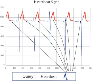
- heartbeat, chest volume, and blood oxygen concentration - are recorded in the time series storage system [3]. There are many open problems regarding the apnea patient datasets. One problem is to find different signals affect each other. Another problem is to determine how episodes of sleep apnea can be predicted from the preceding data recorded by other patients. Searching or comparing a new patient data against the previous dataset is a basic problem for all analysis steps. It is hard to locate an input pattern within datasets because each dataset collected from individual patients greatly varies in size and pattern.
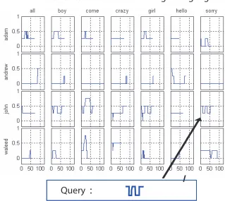
In this paper, we will first begin with subsequence matching of a single channel time series and then extend it to subsequence matching of a multivariable time series. One of the basic problems in handling time series data is locating a pattern of interest from the long sequence of input data [4–6]. The sequence matching problem has two major components: whole sequence matching and subsequence matching. Whole sequence matching involves finding, within the dataset, all sequence entries whose lengths are equal to the query length within the similarity threshold specified by the user. For example, Figure 1.2 illustrates the way the whole sequence matching works to find out how the orientation of the palm of the Australian Sign Language signers is traced for the duration of several different words [7]. Each word of a different signer is of the same length and is searched for a given query.
:
:
Query
:
Palm Orientation of Australian Sign Language
l
a
n
g
i
S
t
a
e
b
t
r
a
e
H
:
y
r
e
u
Q
H
e
a
r
t
b
e
a
t
G
0 2000 4000 6000 8000 10000 12000
0 200 400 600 800 1000 1200 1400 1600 1800 2000
0 50 100 −2 0 2 Cha nnel1
0 50 100 −2
0 2
Cha
nnel2
0 50 100 −2
0 2
Cha
nnel3
0 50 100 −2
0 2
Cha
nnel4
0 50 100 −2
0 2
Cha
nnel5
0 50 100 −2 0 2 Cha nnel6 Query
0 50 100 150 200 250 300 350 400 −2
0 2
0 50 100 150 200 250 300 350 400 −2
0 2
0 50 100 150 200 250 300 350 400 −2
0 2
0 50 100 150 200 250 300 350 400 −2
0 2
0 50 100 150 200 250 300 350 400 −2
0 2
0 50 100 150 200 250 300 350 400 −2
0 2
Data
Evaporator Data
on the whole sequence matching problem [4, 8, 9]. While applying whole sequence matching techniques to the subsequence matching can be possible through the GEMINI [5] framework, the application is not straightforward when non-Euclidean distance measures are used. The Euclidean distance measure is sensitive to noise and, due to the irregular nature of the data in sequence applications (e.g., moving object trajectories, query-by-humming, and etc.), non-Euclidean measures are often more desirable. The non-non-Euclidean distance measures such as Dynamic Time Warping (DTW) and Longest Common Subsequence (LCS) address some of the problems that are characteristic of the Euclidean distance [8, 10].
In this work, we propose an efficient index searching framework for subsequence matching usingLCS. We chooseLCSbecause it is known to be more robust against the noise in the data thanDTW [11, 12]. Furthermore, no separate normalization process is needed to overcome the difference of base unit of multivariable time series. To the best of our knowledge, no previous work has considered LCS in the context of subsequence matching. We make the following contributions:
• We have proposed a subsequence matching framework that employs a non-Euclidean distance measure usingLCS. The result is a more intuitive matching performance.
• We have formally introduced criteria to prune the search space when we use a time series index with theLCSsimilarity function.
adjacent windows are queried and aggregated in order to improve the pruning power of the index.
• We have proposed a new index search scheme that enables us to skip unnecessary simi-larity computations of the consecutive matching subsequences.
Chapter 2
Background and Related Work
2.1 Notational Conventions
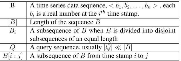
In order to state the problem and concepts clearly, we define some notations and terminolo-gies in Table 2.1. In our work, we assume that a time series is a sequence of real numbers and each real number element is collected from a sensor device. A subsequence is a subset of a time series in contiguous time stamps.
Table 2.1: The Basic Notation
B A time series data sequence,< b1, b2, . . . , bn>, each
bi is a real number at theithtime stamp.
|B| Length of the sequenceB
Bi A subsequence ofB whenB is divided into disjoint
subsequences of an equal length Q A query sequence, usually|Q| ¿ |B|
Query, Q
FRM Subsequence Matching
Data, B
(c) Index Matching Sliding Windows on Data (a)
(b)
(d)
(e) Dual Match Subsequence Matching
(f) Index Matching
Sliding Windows on Query
Query, Q
FRM Subsequence Matching
Data, B
(c) Index Matching Sliding Windows on Data (a)
(b)
(d)
(e) Dual Match Subsequence Matching
(f) Index Matching
Sliding Windows on Query
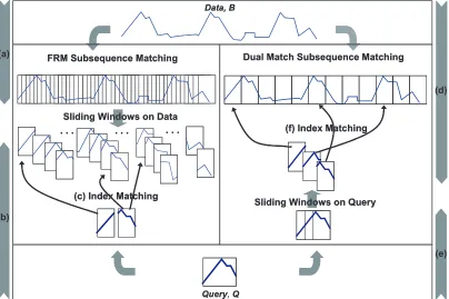
Figure 2.1: Two Subsequence Matching Frameworks
2.2 Subsequence Matching Framework (Dual Match vs. FRM)
There are two subsequence matching frameworks: FRM [5]1and Dual Match [6]. Both of
the matching processes are illustrated in Figure 2.1. Letnbe the number of data points andw be the size of an index window. In FRM, the data sequence is divided inton−w+ 1sliding windows. Figure 2.1 (a) shows the FRM indexing step. Every window overlaps with the next window except for the first data point. QueryQ is divided into disjoint windows, Figure 2.1 (b), and each window is to be matched against the sliding windows of the data sequence, Figure 2.1 (c). In the Dual Match framework, the data sequence is divided into disjoint windows, like in Figure 2.1 (d), and part of the query in its sliding window is matched to the data indexes,
Figure 2.1 (e) and (f). Since the Dual Match does not allow any overlap of the index windows, it needs less space for an index, and consequently spends less index searching time than FRM. Through the index matching, we get a set of candidate data for the matching, and the actual similarity or distance is computed. Since the length of the data is usually very long, the Dual Match framework reduces the indexing efforts. We employ the Dual Match as our indexing scheme.
2.3 Dual Match Subsequence Matching with Euclidean
Dis-tance
Dual Match consists of the following three steps:
• First, in the indexing step, data is decomposed into disjoint windows and each window is represented by a multi-dimensional vector. They are stored in a spatial index structure like an R-tree [13] or R*-tree [14].
• Lastly, depending on the positions of the matching sliding windows, whole matching intervals are determined and actual similarities are computed.
2.4 Non-Euclidean Distance
DTW
and
LCS
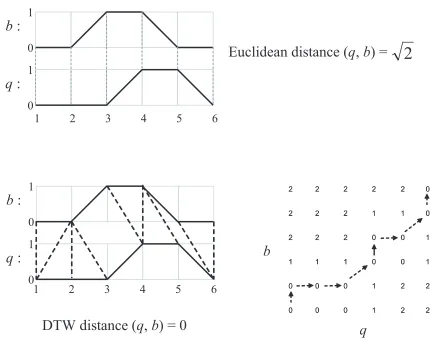
Non-Euclidean similarity measures, such asDTW [12, 15–18] andLCS[10, 19], are useful when we are comparing two time series data sequences that share patterns similar in shapes but irregular in size. Both use dynamic programming algorithms to compute optimal value based on a recursive definition of the solution [16–18]. DTW is an algorithm used to find warping paths of the two time series by computing minimum accumulative distance. The cumulative distance of the two time series sequence is defined as below.
Definition 1 [10] Let Q=< q1, q2, ...qn > be a query and B=< b1, b2, ...bn > be a data
subsequence of time series. The cumulative distanceρi,j is defined asρi,j(Q, B) =d(qi, bj) +
min(ρi−1,j, ρi,j−1, ρi−1,j−1). Then,DT W(Q, B) =ρ|Q|,|B|.
DTWwas introduced to the time series research community by [15]. Figure 2.2 is an exam-ple ofDTW computation. It also comparesDTW to the Euclidean distance of two sequences. This original DTW algorithm has a greater time complexity than the popular Euclidean dis-tance function. DTW hasO(n2)time complexity when two time series are of the same length
n. It is reducedO(δn)by restricting the greedy algorithm to search minimum distance within
opti-Example sequences:
b
: <0,0,1,1,0,0>,
q
: <0,0,0,1,1,0>
Euclidean distance (
q
,
b
) =
b
:
q
:
1 0 1 01 2 3 4 5 6
2
DTW distance (
q
,
b
) = 0
1 0 0b
:
q
:
2 2 1 0 0 0 2 2 1 0 0 0 1 0 0 1 1 1 1 0 0 2 2 2 0 1 1 2 2 2 0 2 2 2 2 2 2 2 1 0 0 0 2 2 1 0 0 0 1 0 0 1 1 1 1 0 0 2 2 2 0 1 1 2 2 2 0 2 2 2 2 2q
b
1 2 3 4 5 6 1
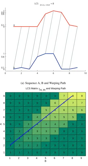
mal warping path is decided byδ. Another popular shape of theδrestriced area is the Itakura band [21]. It has a diagonal diamond shape [21]. We chose the Sakoe-Chiba band for the ease of computation. LCS andDTW share the same dynamic programming procedure to compute the optimal warping path within the δ time interval. We chose LCSas our distance function and the definition is given below.
Definition 2 [10] Let Q=< q1, q2, ...qn>be a query and B=< b1, b2, ...bn >be a data
subse-quence of time series. Given an integerδand a real number 0< ² <1, we define the cumulative
similarityγi,j(Q, B)or γi,j as follows:
γi,j =
0, if i, j = 0
1 +γi−1,j−1 if|qi−bj| ≤²
and|i−j| ≤δ
max(γi,j−1, γi−1,j) otherwise
LCSδ,²(Q, B) =γ|Q|,|B|
0 2 4 6 8 10 0
0.1 0.8 1 0 0.1 0.8 0.91
LCS
[δ=2,ε =0.2] = 8
A
B
(a) Sequence A, B and Warping Path
1 2 3 4 5 6 7 8 9
1 2 3 4 5 6 7 8 9
1 1 1 0 0 0 0 0 0
1 2 2 2 0 0 0 0 0
1 2 3 3 3 0 0 0 0
0 2 3 3 3 3 0 0 0
0 0 3 4 4 4 4 0 0
0 0 0 4 5 5 5 5 0
0 0 0 0 5 6 6 6 6
0 0 0 0 0 6 7 7 7
0 0 0 0 0 0 7 8 8
B
A
LCS Matrix γ
|A|, |B| and Warping Path
(b) Sakoe-Chiba Band and an Optimal Warping Path inLCSComputation Martix
0 5 10 15 20 25 30 75
80 85
E uclidean = 59.1208
0 5 10 15 20 25 30
DT W = 8.4745
0 5 10 15 20 25 30
75 80 85
0 5 10 15 20 25 30
75 80 85
E uclidean = 59.1208
0 5 10 15 20 25 30
DT W = 8.4745
0 5 10 15 20 25 30
75 80 85
0 5 10 15 20 25 30
75 80 85
E uclidean = 59.1208
0 5 10 15 20 25 30
DT W = 8.4745
0 5 10 15 20 25 30
75 80 85
0 5 10 15 20 25 30
70 75 80 85
E uclidean = 177.4743
0 5 10 15 20 25 30
DT W = 93.696
0 5 10 15 20 25 30
0 5 10 15 20 25 30
70 75 80 85
E uclidean = 177.4743
0 5 10 15 20 25 30
DT W = 93.696
0 5 10 15 20 25 30
After inserting a noise* Before inserting a noise*
[δ=5,ε=1]
L C S[[δδ=5,=5,εε=1]=1]= 25 L C S[[[δδδ=5,=5,=5,εεε=1]=1]=1]= 24
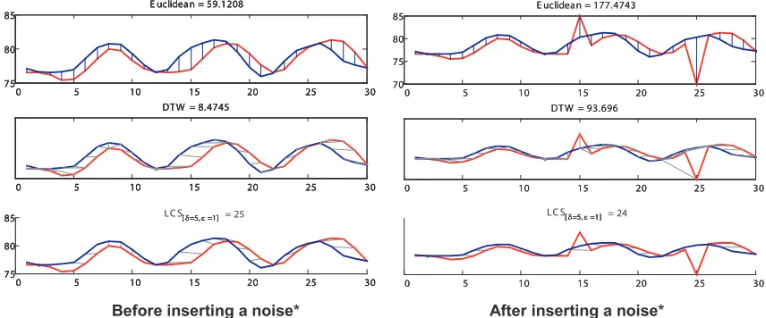
Figure 2.4: Euclidean,DTW andLCSWhen Noise Involved
boxes in light color in theLCSwarping path matrix of Figure 2.3(b) represent a Sakoe-Chiba band [20].
LCS is known to be robust to the noise since it does not count the sequence values out of the range, ². In Figure 2.4, three distance functions are compared by an example. LCS was not affected by noise as much as the other two distance functions. An alternative approach to the noise problem is to use outlier detection algorithms in the pre-processing stage. It helps subsequence matching by removing extreme values even though we use distance functions that are not strong against the noise. However, extra time is required to scan the data in order to get a correct statistics or analysis to identify outliers. [22–24]
2.5 Optimal Bounding for Index Matching
and the query MBE in PAA (Piecewise Aggregate Approximation) representation is a lower bound for theDTW distance between the data and the query. MBE is a Minimum Bounding Envelope that covers all the possible matching points. Enhancing this indexing method of [8], a more efficient index matching scheme was developed by representing a query of the average values of the MBRs in [9]. [10] introducedLCSto the whole sequence matching problem. The number of intersecting time stamps of MBRs is an upper bound for theLCS similarity. This work, however, is proposed not just for the subsequence matching problem but also for the whole sequence matching usingLCS.
2.6 Sequence Alignment
Subsequence matching is similar to the sequence alignment in bioinformatics in that both compare two different sequences. The sequence alignment is used to arrange two DNA or RNA sequences which consist of a small number of characters such as A,T,C and G. By identifying similar regions of two different sequences, researchers try to explain functional or evolutionary relationships of sequence owners. Depending on the number of sequences in a comparison, se-quence matching is categorized into piecewise alignment and multiple sese-quence alignment. In the piecewise alignment, there are two approaches: global alignment and local alignment. The Needleman-Wunsch algorithm [29] is a global sequence alignment method. It is a dynamic programming algorithm that computes the similarity of two sequences. Different from LCS
sequences reset the alignment. Matching (or alignment) is restarted whenever the algorithm encounters unmatched subsequences. The Smith-Waterman algorithm [30] is a popular lo-cal alignment method that employs negative penalty scoring system. Basic Local Alignment
Search Tool (BLAST)[31, 32] is one of the most useful algorithms for genomists to compare
amino-acid sequences or DNA sequences. BLAST is based on the Smith-Waterman algorithm and it is modified by heuristics to enhance computational performance.
2.7 Other Related Work
Chapter 3
Subsequence Matching with
LCS
Using
Dual Match Index in Single Channel
3.1 Problem Statement
The purpose of the subsequence matching is to find subsequences similar to the given query sequence. A subsequence matching framework with the Euclidean distance has been already developed as we stated in the previous section. However, to the best of our knowledge, many things have not yet been considered when applying a non-Euclidean function to the subse-quence matching. We need to improve the index search performance, and we need to provide an index matching criteria that avoids expensive computations caused by non-Euclidean mea-sures.
0 50 100 150 200 250 300 350 −40
−20 0 20 40
Matching Subsequences Query, Q
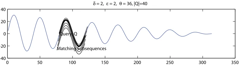
δ = 2, ε = 2, θ = 36, |Q|=40
Figure 3.1: Matching Subsequences in Subsequence Matching
matching subsequences for a query sequenceQin terms ofLCSδ,².
Definition 3 Let Q=< q1, q2, ...qm >be a query and B=< b1, b2, ...bn>be a data subsequence
of time series. Given an integerδ, a real number 0< ² <1 and user defined similarity threshold
θ, we define thematching subsequences,M ={B[i:j]|LCSδ,²(Q, B[i:j])≥θ}
We restrict the scope of our work to searching for the longest possible matching subse-quences of the length|Q|+ 2δ. Finding all the matches of all the lengths with a non-Euclidean measure is time-consuming. It makes sense to find the longest matching subsequences since they also include matching subsequences shorter than |Q|+ 2δ. It is possible to search for shorter matching subsequences after the search process for the longest ones has been com-pleted. In Figure 3.1, all of the matching subsequences of the longest length, |Q|+ 2δ, are demonstrated in grey lines.
Problem : Find all matching subsequences B[i : j] of the length |Q| + 2δ for data sequenceB, and queryQsuch that the similarityLCSδ,²(Q, B[i:j])is no less than s% of the
|Q|, s
100|Q|.
Data Query
[δ=8,ε =0.15]
= 32
0 10 20 30 40 50
= 19 Similarity
[δ=8,ε =0.15]
Similarity
0 10 20 30 40 50
Data Query
(a) Aligned to the left (b) Aligned to the center
Figure 3.2: Alignment withLCSwhen|Query|= 32 and|Data|= 48
• Index pruning criteria (bounding value) is computed to obtain candidates withLCS with-out missing correct matches.
• When it comes to the index use, the number of candidates is decreased by summing up the index search results.
• Adjacent matching intervals are efficiently skipped by observing theLCSmatrix, which allows more expensive similarity computations to be avoided.
3.2 Linear Search and Skipping
LCS
Computation
3.2.1 Alignment in
LCS
When we compare the query Qto a candidate data subsequence of the length |Q|+ 2δ, we align the query in the middle of each candidate as illustrated in Figure 3.2 (b). In the case of the whole sequence matching, alignment is not a problem since the query and data are of the same length. However, in our subsequence matching, we need to locate the query in the candidate subsequence. If we align the query to the left side of a candidate, we cannot find a correct subsequence. In Figure 3.2(a), a shorter query is not matched well to the longer data when aligned to the left. The right side of the query cannot be compared with the data since the δ is not big enough to cover the matching points of the data. A larger δ needs a heavier similarity computation. Figure 3.2 (a) shows that the query is correctly matched with the same δwhen aligned to the center.
3.2.2 Skipping
LCS
Computation
We can avoid expensive similarity computations of the adjacent subsequences by observing the LCSwarping path and the local constraint, such as the Sakoe-Chiba band. In the subse-quence matching, we can think of the computation matrix as a moving window along the data sequence, as in Figure 3.3.
1 2 3 4 5 6 7 8 1 2 3 4 1 2 3 4 1 2 3 4 Need new computation At least
1 2 3 4 5 6 7 8 1 2 3 4 5 6 7 8
(a) (b) (c)
Data B Query
Q
Sakoe-Chiba band
1 2 3 4 5 6 7 8
1 2 3 4 1 2 3 4 1 2 3 4 Need new computation At least
1 2 3 4 5 6 7 8 1 2 3 4 5 6 7 8
(a) (b) (c)
Data B Query
Q
Sakoe-Chiba band
Figure 3.3: An Example of SkippingLCSComputation when|Q|= 4 andδ= 1
by a time stamp. The Sakoe-Chiba band still includes the warping path. In this case, we do not have to compute theLCS(Q, B[2 : 7])since the dynamic programming finds a maximum warping path in the Sakoe-Chiba band and theLCS(Q, B[2 : 7])must be larger than or equal to 4. In Figure 3.3 (c), we need to compute LCS(Q, B[3 : 8]) since only one warping path remains there.
We can skip a computation of a sliding window by tracing the warping path. If we find that the Sakoe-Chiba band of the current LCS matrix includes the previous warping path greater than or equal to the user-defined threshold, then we can skip theLCScomputation. The skip-ping goes until the Sakoe-Chiba band includes a warskip-ping path whose similarity is smaller than the user-defined threshold. It is a useful asset to be used in order to reduce the expensive similarity computation in the subsequence matching where the adjacent window usually has a similar value.
3.3 Indexing
Data is divided into equi-length disjoint windows for the index. Each window is represented by a multi-dimensional vector. That is, data sequence B is divided into equi-length disjoint windows< wi >. Each windowwi consists ofN MBRs. LetN be the dimensionality of the
space we want to index. An MBRrepresents a dimension. N MBRs for a wi is transformed
into −→wi =< (ui1, . . . , uiN),(li1, . . . , liN) >, where uij and lij represent the maximum and
minimum values in thejthinterval ofw
i. −→wiis stored in anN dimensional R-tree. An example
is illustrated in Figure 3.4 (a). In the figure, the data in the first window, w1 =< b1, ..., b9 >
is transformed into−w→1 =<(u11, u12, u13),(l11, l12, l13)>. It is stored in an R-tree as in Figure
3.4 (b).
3.4 Index Matching with
LCS
A queryQis compared first to the index. Qis transformed into anMBEwith the LCSδ,²
function as illustrated in Figure 3.4 (d). Let MBEQ be an MBE forQ. Let the ith sliding
window ofQbevi. It is transformed into−→vi =<(ˆui1, . . . ,uˆiN),(ˆli1, . . . ,ˆliN)>, whereuˆij and
ˆ
lij, respectively, are the maximum and minimum values inMBEQ of thejth MBRof thevi.
This is illustrated in Figure 3.4 (e). SinceMBEQcovers the entire possible matching area, any
point that lies outside theMBEQis not counted for the similarity. The number of intersecting
points betweenB andMBEQ overestimatesLCSδ,²(B, Q)[10]. The number of intersections
MBEQ Query Q Sliding Windows Intersection of B Q
…
N-dimensional R-treew1 v1
N-dimensional R-tree
w1 v1
v1<(u11, u12, u13), (l11, l12, l13)>
MBEQ
^ ^ ^ ^ ^ ^ u^11
u^11
u^12
u^12
u^13
u^13
l13 ^l13 ^ l12 ^l12 ^ l11 ^l11 ^ Data B
…
(c) (d) (e)
(a) (b)
Indexed by disjoint windows
v1 v1
w1: <(u11, u12, u13), (l11, l12, l13)>
w1: <(u11, u12, u13), (l11, l12, l13)>
w1
w1and v1
w1and v1
w2 u12 u11 l13 u13 l12 u21 u22 l22 l21 l11 MBR
…
Decomposed into sliding windows MBE
Qby LCSS d, e
Figure 3.4: Indexing and Index Matching wherew=9 andN=3
3.4 (a) and Figure 3.4 (e).
3.5 Window Sliding Schemes in Index Matching
There are three ways to slide query windows and choose the candidate matching subse-quences: Simple Single Window Sliding, Single Window Sliding, and Multiple Window Slid-ing. We explain each window sliding scheme and show how the the bounding similarity is computed.
3.5.1 Simple Single Window Sliding
Query, Q Query, Q
(a) Simple Single Window
Query, Q Query, Q
(b) Single Window
Query, Q Query, Q
(c) Multiple Window
Figure 3.5: Window Sliding Schemes when|v|=4.
… …
v
?
?
(a) Simple single sliding window
(b) Lost matching points Q B Query’s MBE Sliding Windows For Q Query’s MBE w w v d d … … v ? ?
(a) Simple single sliding window
(b) Lost matching points Q B Query’s MBE Sliding Windows For Q Query’s MBE w w v d d
Figure 3.6: Matching points (connected by dotted lines) are not captured in the index matching usingLCS
We should consider δ on both ends of the query sliding window. In Figure 3.6 (a), a sliding window v of a query Q is matched to a window w of the data sequence B. In actual index matching, some points near the start and end of the queryQcannot be matched to those ofw as in Figure 3.6 (b). The data is just indexed byMBRthat does not considerδtime shift.
is no less than s% of the|Q|, s
100|Q|. Letvbe a sliding window ofQ. The minimum similarity,
θis
θ=|v| −(|Q| − s
100|Q|)−2δ (3.1)
The term,(|Q| − s
100|Q|), for the Equation (3.1) is subtracted from|v|when all the mismatches
can be found in the current window v. The last term 2δ is the maximum possible number of the lost matching points.
3.5.2 Single Window Sliding
When the query length is long enough to contain more than one sliding window, we can use the consecutive matching information as in Figure 3.5(b). Let us assume queryQand matching subsequenceB haveM consecutive disjoint windows,Bi’s andQi’s. If someQiandBi pairs
are not similar, then the other Qj and Bj pairs should be similar, and we can recognize the
B and Qpair as a candidate because ofBj andQj. When all Bi andQi pairs have the same
similarities, we should have the minimum value to establish the candidate for comparison. The
multiPiecesearch [5] is proposed to choose candidates through this process. It is the same for
the Euclidean distance measure. In themultiPiece, the two subsequences,BandQ, of the same length are given, and each can be divided intopsubsequences, each of which is of the length l. d(B, Q) < ² ⇒d(Bi, Qi) < √²p for some1≤i ≤pwhereBi andQi areithsubsequences
of lengthland² > 0. In the case of the Dual Match using Euclidean distance, we can count a candidate if the distance is less than or equal to √²
p.
Similarly, in the case ofLCS,LCSδ,²(B, Q)> 100s |Q| ⇒LCSδ,²(v, Q[i:j])> M|v|−(|Q|−
s
100|Q|)−2δ
for somej−i+ 1 =|v|. So the similarity threshold for single window sliding,θs, is
θs=|v| −
(|Q| − s
100|Q|) + 2δ
M (3.2)
As illustrated in Figure 3.5(b), M consecutive sliding windows are thought to be one large sliding window that might lose the warping path at both ends. The threshold for theM sliding windows is M|v| −(|Q| − s
100|Q|)−2δ, and it is divided by M for one sliding window. If
one of the sliding windows among consecutiveM sliding windows inQis larger than or equal toθs, we can obtain a candidate, and we do not have to do index matching for the remaining
consecutive sliding windows at the same candidate location.
3.5.3 Multiple Window Sliding
In this new window sliding scheme, as illustrated in Figure 3.5(c), the matching results of consecutive sliding windows in a query are aggregated. If we sum up the index matching result fromM consecutive sliding windows, we can obtain fewer false candidates than when we use only one window. LetM be the number of consecutive windows fitted in a queryQ. We vary M to contain the maximum number of sliding windows depending on the left-most window.
8 8 9
8 1
4 2
20 12
v1 v2 v3
Data B
Vector A Query
Q
8 3
w1w2
. . .
wmTemporary vector to store matching results
8 8 9
8 1
4 2
20 12
v1 v2 v3
Data B
Vector A Query
Q
8 3
w1w2
. . .
wmTemporary vector to store matching results
Figure 3.7: Index Matching Result
Q. The index matching results of a query windowvj are placed in a temporary row vector in
Figure 3.7. It is added toA, andAis shifted right. The next matching result forvj+1 is placed
in the temporary row vector. It is added toA, andA is shifted right. In Figure 3.7, we getA such that
A[1] =LCSδ,²(−→v1,w−→1) +LCSδ,²(−→v2,−→w2) +LCSδ,²(→−v 3,−→w3),
A[2] =LCSδ,²(−→v1,w−→2) +LCSδ,²(−→v2,−→w3) +LCSδ,²(→−v 3,−→w4),
...
A[m] = LCSδ,²(−→v1,−−−→wm−2) +LCSδ,²(−→v2,−→wm−1) +LCSδ,²(−→v 3,−→wm).
The shift operations aggregate the consecutive index matching results.
The similarity threshold for multiple sliding windows,θm, is computed as if the consecutive
M windows moved as one.
θm =M|v| −(|Q| −
s
θm is for an aggregate comparison of M consecutive sliding windows, while θs is for one
sliding window.
Using the aggregation of the consecutive index matching information, we can enhance the pruning power of the index. That is, we have fewer false alarms than the single window sliding scheme does. In Figure 3.7, the diagonal sum illustrates the aggregatation of the consecutive index matching results. Ifθs = 8, the first, second, and the fifth diagonals are selected as the
candidates since one of the matches is greater than or equal to 8. However, in the case of the multiple window sliding, ifθm = 20, the fifth diagonal is not a candidate since the sum 12 is
less than 20, so it has fewer false alarms than the single window sliding scheme does.
3.6 Post-Processing and Skipping
3.6.1 Post-Processing
Query, Q
Actual Matching intervals I3
I1 I2
1
2
3
1 2 3
Data, B
Data, B Query, Q
Actual Matching intervals I3
I1 I2
1
2
3
1 2 3
Data, B
Data, B
Figure 3.8: Postprocessing determines the entire lengths of the candidate subsequences
depending on the location of the sliding window in the query.
3.6.2 Skipping the
LCS
Computation
After determining the whole length of the candidate subsequences, skipping theLCS com-putation is applied to reduce the comcom-putational load. Subsequence matching cannot avoid many adjacent matching subsequences where one subsequence is found. By tracing the warp-ing path of the matchwarp-ing subsequences in itsLCSwarping path matrix, we can reduce theLCS
computation.
3.7 Experiment of Single Channel Time Series Dataset
Experiments were conducted on a machine with a 2.8 GHz Pentium 4 processor and 2GB memory using Matlab 2006a and Java. Here are the parameters to run the tests:
• Dataset: We have used 48 different time series datasets1 for evaluation. Each dataset
has a different data length and a different number of channels. We set the length of each to 100,000 by attaching the beginning to the end so that all the datasets have the same length.
• Index: We set the dimension to 8 and MBR size to 4. Determining the sizes of the dimension,MBRand R-tree requires domain knowledge.
• Query: We choose 4 fixed lengths of queries, 100, 150, 180, and 200, so that each length includes 3, 4, 5 and 6 windows. Ten queries for each length are randomly selected from the data sequence.
• Similarity: ²is set to 1%of the data range, andδis set to 2.5%of the|Q|. Similarity threshold S is set to99%of the|Q|.
3.7.1 Different Sliding Schemes and Candidates
We compare the performance of the two different index sliding schemes, namely, the sin-gle window sliding and the multiple window sliding scheme. Figure 3.9 shows the ratios,
# of candidates by single windows sliding
# of candidates by multiple windows sliding for different lengths of queries of each dataset. Ratios greater
than one means the multiple window sliding scheme generates fewer candidates than those of the single window sliding scheme. The multiple window sliding scheme has fewer false alarms than the single window sliding scheme in the tests. The ratio varies from 1 to 140. The multiple sliding window scheme generates candidates only 1
140 of the single window sliding scheme in
100150 180200 1 3 5 7 9 11 13 15 17 19 21 23 25 27 29 31 33 35 37 39 41 43 45 47 0 20 40 60 80 100 120 140 Query Length 25:powerplant 26:shuttle 27:attas 28:soiltemp 29:pHdata 30:Realitycheck 31:earthquake 32:ballbeam 33:flutter 34:balloon 35:glassfurnace 36:wind 37:evaporator 38:TOR95 39:network 40:synthetic control 41:burstin 42:leaf all 43:darwin 44:motorCurrent 45:pgt50 alpha 46:robot arm 47:twopat 48:EEG heart rate Candidate Ratio for ( Multipiece Single / Multipiece Multiple )
(ε = 0.01, δ = 0.025, S = 99%, Dim = 8, MBR_size = 4)
Data File 1:Fluid dynamics 2:tickwise 3:tide 4:steamgen 5:buoy sensor 6:random walk 7:power data 8:winding 9:infrasound beamd 10:foetal ecg 11:koski ecg 12:chaotic 13:cstr 14:eeg 15:sunspot 16:dryer2 17:standardandpoor500 18:spot exrates 19:memory 20:greatlakes 21:leleccum 22:ocean shear 23:ocean 24:speech Candida te Ra ti
o for ( Mult
ipiece
Single / Mult
ipi ece Mul tipl e )
100 150 180 200 1
2 3 4 5 6 7
Median Candidate Ratio of Single Window/Multiple Window (ε = 0.01, δ = 0.025, S = 99%, Dim = 8, MBR_size = 4)
Query Length, |Q| Median
Ratio
Figure 3.10: Summary of Candidate Ratio in Figure 3.9
Figure 3.10 shows the median values from the Figure 3.9 for each length of the queries. Figure 3.10 summarizes how much the performance is improved as the length of the query gets longer in all of the datasets. It demonstrates that as the length of a query gets longer to include more index windows, fewer false alarms occur in the multiple window sliding than in the single window sliding.
Best 3
0 50 100 150 200 250 300 350 400 450 500
−1 0 1
fluid dynamics
0 50 100 150 200 250 300 350 400 450 500
2.082 2.1027
tickwise
0 50 100 150 200 250 300 350 400 450 500
−31.8965 55.0042
tide
Worst 3
0 50 100 150 200 250 300 350 400 450 500 66.615
560.083
network
0 50 100 150 200 250 300 350 400 450 500 23.512
43.6161
synthetic control
0 50 100 150 200 250 300 350 400 450 500 0.0673575
2.3878
burstin
100 150 180 200 1 3 5 7 9 11 13 15 17 19 21 23 25 27 29 31 33 35 37 39 41 43 45 47 0 0.1 0.2 0.3 0.4 Data File Tightness for Single Sliding
(ε = 0.01, δ = 0.025, S = 99%, Dim = 8, MBR_size = 4)
# of Es
tim at ed Si mi la rit y /
# of Tr
ue Simil ar ity 100 150 180 200 1 3 5 7 9 11 13 15 17 19 21 23 25 27 29 31 33 35 37 39 41 43 45 47 0 0.1 0.2 0.3 0.4 Data File Tightness for Multiple sliding (ε = 0.01, δ = 0.025, S = 99%, Dim = 8, MBR_size = 4)
37:steamgen 38:sunspot 39:synthetic control 40:tide 41:TOR95 42:twopat 43:wind 44:winding 45:koski ecg # o f Es tima ted Si mil ar
ity / #
of Tru e Sim ila rity 25:pgt50 alpha 26:pHdata 27:powerplant 28:power data 29:random walk 30:Realitycheck 31:robot arm 32:shuttle 33:soiltemp 13:Fluid dynamics 14:flutter 15:foetal ecg 16:glassfurnace 17:greatlakes 18:infrasound beamd 19:leaf all 20:leleccum 21:memor 1:attas 2:ballbeam 3:balloon 4:buoy sensor 5:burstin 6:chaotic 7:cstr 8:darwin 9:dr er2 100150 180200 1 3
5 7911 1315 1719 2123 25272931 3335 3739 4143 4547 0 0.2 0.4 0.6 0.8 Data File Goodness for Single Sliding
(ε = 0.01, δ = 0.025, S = 99%, Dim = 8, MBR_size = 4)
# of Ca
nd
id
at
es / # of T
rue Matches
100150180200 1 35 7
911 1315 1719 21232527 2931 3335 3739 4143 4547 0 0.2 0.4 0.6 0.8 Data File
Goodness for Multiple sliding (ε = 0.01, δ = 0.025, S = 99%, Dim = 8, MBR_size = 4)
# of Ca
nd
id
at
es / # of True Matches
3.7.2 Goodness and Tightness
Goodness and tightness are metrics that show how well the index works [8].
Goodness= # of all true matches
# of all candidates (3.4)
T ightness= Sum of all true similarity
Sum of all estimated similarity (3.5)
Goodness shows how much the index reduces the expensive computations. Tightness shows how close the estimated values are to the actual values in indexing [8]. If the tightness is 1.0, then it means that the estimation is perfect. In Figure 3.12, the multiple sliding window scheme shows greater goodness and tightness than that of the single window sliding scheme.
3.7.3 Improving Performance by Skipping Similarity Computations
Figure 3.13 shows how effective the skipping of the similarity computation is. The chart demonstrates that we can avoid many similarity computations as the length of the query gets longer.
1 4 7 10 13 16 19 22 25 28 31 34 37 40 43 46 0 0.2 0.4 0.6 0.8 200 Query Length 180 150 100
Skipped Matching Ratio for All Candidates (ε = 0.01, δ = 0.025, S = 99%, Dim = 8, MBR_size = 4)
Data File
# Skipe
d / # Candid
ate 37:glassfurnace 38:pgt50 alpha 39:robot arm 40:soiltemp 41:darwin 42:balloon 43:earthquake 44:twopat 45:evaporator 46:EEG heart rate 47:network 48:burstin 25:dryer2 26:power data 27:steamgen 28:buoy sensor 29:foetal ecg 30:koski ecg 31:sunspot 32:speech 33:motorCurrent 34:leaf all 35:synthetic control 36:flutter 13:powerplant 14:TOR95 15:spot exrates 16:attas 17:leleccum 18:chaotic 19:wind 21:pHdata 22:eeg 23:tide 24:winding 1:ballbeam 2:cstr 3:greatlakes 4:infrasound beamd 5:memory 6:ocean 7:ocean shear 8:random walk 9:Realitycheck 10:shuttle 11:standardandpoor500 12:tickwise 20:Fluid dynamics
3.7.4 Runtime
We compare the performance of FRM, single window sliding dual match and the multiple sliding window Dual Match in CPU time. 10 randomly selected queries are searched against 48 datasets. Experiments are done for four different lengths: 100, 150, 180 and 200. Figure 3.14 shows median CPU times of 10 runs of subsequence matching using three different methods for each query length. It shows that in most cases, multiple sliding window scheme performs better than FRM and single sliding windows. FRM spent much more time on searching an R-tree than Dual Match method did. In the case the data size is nand index window size is
1: Fluid_dynamics 2: tickwise 3: tide 4: steamgen 5: buoy_sensor 6: random_walk 7: power_data 8: winding 9: infrasound_beamd 10: foetal_ecg 11: koski_ecg 12chaotic 13: cstr 14: eeg 15: sunspot 16: dryer2 17: standardandpoor500 18: spot_exrates 19: memory 20: greatlakes 21: leleccum 22: ocean_shear 23: ocean 24: speech 25: powerplant 26: shuttle 27: attas 28: soiltemp 29: pHdata 30: Realitycheck 31: earthquake 32: ballbeam 33: flutter 34: balloon 35: glassfurnace 36: wind 37: evaporator 38: TOR95 39: network 40: synthetic_control 41: burstin 42: leaf_all 43: darwin 44motorCurrent 45pgt50_alpha 46: robot_arm 47: twopat 48: EEG_heart_rate
1 3 5 7 9 11 13 15 17 19 21 23 25 27 29 31 33 35 37 39 41 43 45 47
0 500 1000 1500 2000 2500 Data File CPU t ime (second)
CPU time : Single Window Sliding vs. Multiple Window Sliding
FRM
Single Windlw(Dual Match) Multiple Window(Dual Match)
1 3 5 7 9 11 13 15 17 19 21 23 25 27 29 31 33 35 37 39 41 43 45 47
0 1000 2000 3000 4000 5000 Data File CPU t ime (second ) |Q| =180 FRM
Single Windlw(Dual Match) Multiple Window(Dual Match)
1 3 5 7 9 11 13 15 17 19 21 23 25 27 29 31 33 35 37 39 41 43 45 47
0 500 1000 1500 2000 2500 3000 3500 Data File CPU t ime (second ) |Q| =150 FRM
Single Windlw(Dual Match) Multiple Window(Dual Match)
1 3 5 7 9 11 13 15 17 19 21 23 25 27 29 31 33 35 37 39 41 43 45 47
0 1000 2000 3000 4000 5000 Data File CPU t ime (second ) |Q| =200 FRM
Single Windlw(Dual Match) Multiple Window(Dual Match)
(ε = 0.01, δ = 0.025, S = 99%, Dim = 8, MBR_size = 4)
|Q| =100
1000 150 180 200 100
200 300 400 500 600
Query Length
CPU t
ime
(second)
Median CPU time : Single Window Sliding vs. Multiple Window Sliding (ε = 0.01, δ = 0.025, S = 99%, Dim = 8, MBR_size = 4)
FRM
Single Windlw(Dual Match) Multiple Window(Dual Match)
Chapter 4
Multivariable Subsequence Matching
4.1 Introduction
10 20 30 −1
0 1
x
10 20 30 −1
0 1
y
10 20 30 −1
0 1
z
10 20 30 −1
0 1
roll
10 20 30 −1
0 1
thumb
10 20 30 −1
0 1
index
10 20 30 −1
0 1
middl
e
10 20 30 −1
0 1
rin
g
0 30 60 90 120 150 180 210 240 270 300
−1 0 1
0 30 60 90 120 150 180 210 240 270 300
−1 0 1
0 30 60 90 120 150 180 210 240 270 300
−1 0 1
0 30 60 90 120 150 180 210 240 270 300
−1 0 1
0 30 60 90 120 150 180 210 240 270 300
−1 0 1
0 30 60 90 120 150 180 210 240 270 300
−1 0 1
0 30 60 90 120 150 180 210 240 270 300
−1 0 1
come girl man maybe mine name read right science thank −1
0 1
x OP tG k
channel time series data. With the advancement of the sensor technology, many applications require tracing a large number of channels from various sources.
Time series data is usually stored in a back-end intelligence module to analyze the prop-erties of the data. The multivariable time series data is also fed as input to some online appli-cations monitoring real-time events based on the back-end analysis. Unfortunately, however, traditional data mining solutions are not directly applicable to the sensor network applica-tion framework. Tradiapplica-tional techniques focus on rather static collecapplica-tions of records containing mainly discrete values, while in sensor network applications, data is an unbounded stream of continuous values. Furthermore, characteristics of data instances are also different. A record in sensor stream data typically contains values representing particular sensor readings at a given point in time. Unlike the traditional databases, the records in this environment have temporal locality; for example, the current sensor readings are likely to be similar to the ones observed recently rather than to the ones monitored a long time ago. These differences pose substantial challenges to the traditional data management techniques, enough to force a paradigm shift in the long-established data management standards.
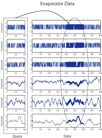
The use of multiple channels of signals would increase the accuracy of the security sys-tem even though multivariable time series requires complex analysis. For example, in sign language recognition, movements of the body parts are captured in a multivariable time series data. The orientation of a palm, its angles as well as the positions of fingers, wrists, and arms are represented in a time series for recognition. Figure 4.1 shows an example of a search of multivariable time series in Australian Sign Language [7]. The data has 8 channels (x, y, z position of a hand, orientation of a palm, and the folding degree of 4 fingers). In the figure, data (to be searched) is a time series of 10 different sign words. Each word comes from one of the 20 different signers. The query is the sign word, ”girl.” Subsequence matching in this multivariable time series is to locate the query sign word in the data. In this example, data is a kind of a sign language sentence, although the actual one is more complicated than this one, since there is a pause between two words and the length of each word is not as regular as the provided example.
We chose LCSin definition 2 as our non-Euclidean measure to run similarity matching to overcome the Euclidean measure. If we apply LCS to each channel of a multivariable time series data, we do not have to perform extra computations for normalization or weighting to avoid problems from different basis units of each channel.
We avoid many expensive LCS computations in subsequence matching by observing the computation matrix. LCSrequires expensive computation;O(|Q|2), when queryQis compared
Table 4.1: The Notation for Multivariable Time Series B A multivariable time series data sequence, <
b1,1, b1,2, . . . , b2,1, b2,2, . . . >, eachbi,j is a real
num-ber at theithchannel andjthtime stamp.
B[i,:] ithchannel of data
B[:, j :k] a window of data fromjthframe tokthframe
Q A query sequence, we assume that all channels in Q are of the same length.
subsequences are computed through an inexpensive operation. In the following sections, we will explain how to compute and reduce candidate matching subsequences by applying our proposed method to the multivariable time series data. We will also validate our proposed method through the experiments carried out on 14 multivariable datasets.
4.2 Notational Conventions
Multivariable time series data is expressed in two dimensions, value and time, in several streams. Each stream is called achannel and it represents a feature or attribute of a temporal event in real numbers. These values are recorded in regular time intervals. A time stampis a time point when a set of values of all channels is recorded. The set of values for all channels at a time stamp is aframe. Awindowis a set of frames. The number of frames in a window is the size of the window. All terms are illustrated in Figure 4.2.
l e n n a h C
e m a r F w
o d n i W
0 1 2 3 4 5 6 7 8 9 01 1112131415161718192021222324252627282930 ]
: , 1 [ B
e m i T
V
a
lue
s
] : , 2 [ B
] : , 3 [ B
4.3 Problem Statement
We apply the proposed subsequence matching method in a single channel dataset to the multivariable time series data. We generalize the definition of matching subsequences in Defi-nition 3 for multivariable time series withLCSδ,²i.
Definition 4 Let Q=< q1,1, q1,2, ...qm,n >be a query and B=< b1,1, b1,2, ... >be a data
sub-sequence of time series ofm channels of finite length. Given an integerδ, a real number 0<
²i <1 for eachithchannel and user defined similarity thresholdθ, we define thematching
sub-sequences, M = {B[:, j : k]|LCSδ,²i(Q, B[:, j :k]) ≥ θ}, where LCSδ,²i(Q, B[:, j :k]) =
P
1<i<nLCSδ,²i(Q[i,:],B[i,j:k])
m }
Problem: Find all matching subsequences B[:, j : k] of the length|Q|+ 2δ for data se-quenceB and queryQsuch that the similarity LCSδ,{²i}(Q, B[:, j :k])is no less than S% of
the|Q|, S
100|Q|.
Solution Road MapHere is a road map of solutions to the problem:
• Index pruning criteria (bounding value) is computed and applied to each channel.
• Candidates from the index matching process are chosen by summing up the contiguous index search results.
A window of 8 MBRs
Figure 4.3: An Example of an Index that ShowsMBRsand Windows
4.4 Indexing for Multivariable Time Series
Subsequence matching in multivariable time series data begins by indexing each channel of data into separate R-trees. If there aremchannels, we needmseparate R-trees. Each channel has its own error range to determine similarity. That is, ith channel has its own ²
i for LCS
similarity depending on the application context. All channels share the sameδ.
Data is divided into equi-length disjoint windows for the index. Each window is represented by a multi-dimensional vector. That is, data sequence B is divided into equi-length disjoint windows < wi(k) >, ith window of the channel k. It consists of N MBRs. Let N be the
for awi(k), is transformed into
−−−→
wi(k) =< (ui1, . . . , uiN),(li1, . . . , liN) >k, whereuij andlij
represent the maximum and minimum values in thejthinterval ofw
i(k). −→wiis stored in anN
dimensional R-tree for channelk, R-tree(k).
4.5 Index Matching in Multivariable Time Series
A query is represented byMBE-MBRs. Each channel of the queryQis transformed into an
MBE, and one or more sliding windows are chosen depending on window sliding schemes. We obtain m MBEs from the m channels of the query Q, and each MBE is divided into separateMBRs of the chosen sliding window. We compare this transformed query against the data using the Dual Match index. Figure 4.4 illustrates index matching steps in multivariable time series.
Formally, let MBEQ(j) be an MBE for Q[j,:], jth channel of Q. Let the ith sliding
window of Q[j,:]be vi(j). It is transformed into
−−→
vi(j) =< (ˆui1, . . . ,uˆiN),(ˆli1, . . . ,ˆliN) >j,
whereuˆikandˆlik, respectively, are the maximum and minimum values inMBEQ(j)of thekth
MBRof the−−→vi(j).
MBEQ(j)covers whole possible matching areas usingLCS. Any point that lies outside the
MBEQ(j)is not counted for the similarity. The number of intersecting points betweenB[j,:
] and MBEQ(j) overestimates LCSδ,²j(B[j,:], Q[j,:]) [10]. So,
P
jLCSδ,²j(B[j,:], Q[j,:])
7 4
Channel 1
Sliding window1
w
1w2w3…
20 12
18 8
a candidate
Not a
candidate A candidate if average >= ɂ Temp sum of Channel 1
Sliding window 1
v 1 v 2 v 3
19 10 Average of all channel
for sliding window1
average ˻ ɂ
average < ɂ
Query
Data
Sliding window 2
Sliding window 3
7 4 6 4 20 12 6 3 Channel 2 Sliding window1 w 1w2w3…
v 1 v 2 v 3 Data 6 3 6 2 18 8 Temporary vectors 1 2 3
Temp sum of Channel 2 *Assume that threshold ɂis 16.
Figure 4.4: An Example of Multivariable Subsequence Matching
We apply one sliding window to all channels of query. In the figure, a windowqiof query
Qis searched in R-tree indexes to find estimated matching values. These values are stored in a temporary vector like 1°in figure 4.4. The individual matching process of each channel is the same as the one for the single channel data.
We use the sameθs and θm depending on the window sliding schemes. These were
com-puted in the previous chapter.
Temporary vectors of a channel are diagonally aggregated into a vector, temp sum of a channel, labeled 2°in Figure 4.4. In the 2-channel example of Figure 4.4, the first element of the temporary vector in channel 1 is a sum of 7 + 7 + 6.
results. Only the vector elements greater than or equal to the matching threshold,θm orθs, are
considered candidates.
4.6 Post-processing
Post-processing determines the whole length of the matching subsequence by actual LCS
computation. Candidate subsequences are chosen based on this index matching. If the average value ofLCSsimilarities of all channels are greater than or equal to the threshold ,θsorθm, a
candidate is chosen. If not, the window is not chosen for a candidate. In Figure 4.4, a window that has (12 + 8) / 2 in the result of index matching will be rejected since it is less than the computed threshold 16.
4.7 Skipping with
LCS
for Multivariable Time Series
We can skip one or moreLCScomputations in the neighboring candidates by observing the
4.8 Experiment of Multivariable Time Series Dataset
Here is a brief introduction to the multivariable datasets used in our experimental study and its parameters chosen to run our tests:
• Dataset: We have used 14 different time series datasets 1 for evaluation. Each dataset
has a different length of data and a different number of channels from 2 to 15. We set the length of each to 10,000 by attaching the beginning to the end so that all the datasets are of the same length.
• Index: We set the dimension to 8 and MBR size to 4. Determining the sizes of the dimension,MBRand R-tree requires domain knowledge.
• Query: We chose 4 fixed-lengths of queries, 100, 150, 180, and 200, so that each length
includes 3, 4, 5 and 6 windows. Ten queries for each length are randomly selected from the data sequence.
• Similarity: ²is set to 1%of the data range, andδis set to 2.5%of the|Q|. Similarity threshold S is set to99%of the|Q|.
4.8.1 Different Sliding Schemes and Candidates in Multivariable Time
Series Data
In the first experiment with multivariable time series datasets, we compare the performance of two different index sliding schemes, single window sliding, and multple window sliding,
100 150
180 200
1
3
5
7
9
11
13 0
50
Query Length 8:cstr(3)
9:phone1(8) 10:winding(7) 11:wind(15) 12:steamgen(4) 13:foetal ecg(9) 14:shuttle(6) Candidate Ratio for ( Multipiece Single / Multipiece Multiple )
(ε = 0.01, δ = 0.025, S = 99%, Dim = 8, MBR_size = 4)
Data File 1:evaporator (6) 2:Physiological data B1(3) 3:water(3)
4:buoy sensor(4) 5:phdata(3) 6:greatlakes(5) 7:baloon(2)
( Multipiece Sin
gle
/ Mult
ipiece Multip
le
)
100 150 180 200 1
2 3 4 5 6
Median Candidate Ratio of Single/Multiple (ε = 0.01, δ = 0.025, S = 99%, Dim = 8, MBR_size = 4)
Query Length, |Q| Median
Ratio
Figure 4.6: Summary of Candidate Ratio in Figure 4.5
in the multivariable time series data. By counting the number of candidates, we can correctly compare the performance of two methods independently. For ease of comparison, a ratio of the candidates is computed. Figure 4.5 shows that ratio, # of candidates by multiple windows sliding# of candidates by single windows sliding increases as the length of queries increases for most datasets. The number of channels of a dataset is specified in the legend of the figure. In this experiment, the multiple window sliding scheme has fewer false alarms than the single window sliding scheme. The ratio varies from 1 to 50. In the best case, the multiple sliding window generates candidates only 1
50 of the single window
sliding scheme.
Figure 4.6 shows the median values from Figure 4.5 for each length of the queries. It summarizes the improvement that occurs as the length of the query gets longer when we use the multiple window sliding method. We have fewer false alarms in the multiple window sliding than in the single window sliding as the length of a query gets longer. For the longer query, we have more index windows than for the shorter one, which reduces the chances of getting wrong candidates.
![Figure 1.1: Sleep Apnea: An Example of Time Series Analysis [1], wk :wake, slp:sleep](https://thumb-us.123doks.com/thumbv2/123dok_us/1397337.1172437/15.612.124.516.216.576/figure-sleep-apnea-example-time-series-analysis-sleep.webp)