Dynamic and Aerodynamic Modeling of the Mars Tumbleweed Rover.

ABSTRACT

SHAH, MANTHAN. Dynamic and Aerodynamic Modeling of the Mars Tumbleweed Rover. (Under the direction of Dr. Andre P Mazzoleni).

The conventional wheeled rovers that have landed on Mars are limited by their ability

to operate in a rugged terrain and have been able to cover relatively small portions of

the Martian surface. Their high cost and complexity has demanded a completely new

approach to be taken for the rover design. The Mars Tumbleweed rover is a concept designed

to cheaply and efficiently investigate broad swaths of Mars using the Martian winds for

propulsion. This concept is capable of overcoming the drawbacks of traditional rovers but

it has its own challenges and limitations. Directional control and an effective aerodynamic

design are a few of those design challenges posed by the Mars Tumbleweed rover which

have been addressed in this thesis.

Firstly, as a part of this work, a dynamic model based on the Newton Euler equations of

motion was created to simulate the rolling/sliding motion of the Tumbleweed rover on a flat

terrain. The potential of moving masses for the directional control of the Tumbleweed rover

was demonstrated. The effect of changing the moving mass values on the response of the

system was studied. Also, the performance of the system on varying different parameters

was examined.

As the next step in this research, the aerodynamic characteristics of the Box Kite and the

Tumbleweed Earth Demonstrators (TED) were analyzed using wind tunnel testing. A new

wind tunnel experimental setup was conceptualized and fabricated.CD v s R e curves of all of the above structures helped quantify their aerodynamic properties. On the other hand,

the flow visualization tests helped qualitatively understand their aerodynamics. The outer

structure’s influence on the aerodynamics of the internal Box Kite was also investigated.

of their aerodynamic properties but also on the basis of their dynamic and structural

© Copyright 2019 by Manthan Shah

Dynamic and Aerodynamic Modeling of the Mars Tumbleweed Rover

by Manthan Shah

A thesis submitted to the Graduate Faculty of North Carolina State University

in partial fulfillment of the requirements for the Degree of

Master of Science

Mechanical Engineering

Raleigh, North Carolina 2019

APPROVED BY:

Dr. Kenneth Granlund Dr. Larry M Silverberg

DEDICATION

BIOGRAPHY

Manthan Shah was born and raised in India, where he graduated with his Bachelor’s degree

in mechanical engineering from the University of Mumbai in 2017. Soon after which, he

began pursuing his master’s degree in mechanical engineering at North Carolina State

University in the fall of 2017. From the summer of 2018, he has worked on his master’s

thesis research in the Engineering Mechanics and Space Systems Laboratory (EMSSL) under

ACKNOWLEDGEMENTS

First and foremost, I would like to thank Dr. Mazzoleni for giving me this opportunity of

working on my thesis. Without his invaluable guidance, this thesis would not have been

possible.

I would also like to thank Dr. Granlund and Dr. Silverberg for being a part of my advisory

committee. I sincerely appreciate the support of all my labmates who helped me tackle any

obstacle that came my way.

I cannot thank my parents enough for their constant and unconditional love and support.

Also, I am grateful to all my family and friends whose continual love and support made this

TABLE OF CONTENTS

List of Tables. . . vii

List of Figures. . . viii

Chapter 1 INTRODUCTION. . . 1

1.1 Overview of Mars Exploration . . . 1

1.2 Overview of Wind-Driven Spherical Rovers . . . 3

1.3 Overview of the Mars Tumbleweed Rover . . . 5

Chapter 2 3D TUMBLEWEED ROVER DYNAMICS . . . 8

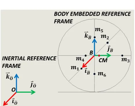
2.1 Reference Frames . . . 9

2.1.1 Inertial Reference Frame . . . 9

2.1.2 Body Embedded Reference Frame . . . 9

2.1.3 Rotation Matrices . . . 10

2.1.4 Direction Cosine Matrix . . . 11

2.1.5 Angular Velocity . . . 11

2.1.6 Euler Parameters . . . 13

2.2 Governing Equations of Motion . . . 14

2.2.1 Forces and Torques Acting on the System . . . 14

2.2.2 Angular Momentum of the System . . . 19

2.3 Solving the Equations of Motion . . . 21

2.3.1 State Space Vector . . . 21

2.3.2 ODE Function . . . 23

2.4 Simulation Results . . . 23

2.4.1 Validation of the Dynamic Model . . . 24

2.4.2 Effect of Varying Different Parameters on the Performance of the Tumbleweed Rover . . . 26

Chapter 3 AERODYNAMICS OF THE BOX KITE . . . 33

3.1 Wind Tunnel Testing . . . 34

3.1.1 Reynolds Number . . . 34

3.1.2 Flow Similarity . . . 35

3.1.3 Wind Tunnel Model . . . 36

3.1.4 Dynamic Pressure . . . 37

3.1.5 Wind Tunnel . . . 37

3.1.6 Force/Moment Balance . . . 38

3.1.7 Experimental Setup . . . 38

3.1.8 Experiment Procedure . . . 41

3.2 Wind Tunnel Results . . . 42

3.2.2 Wind Tunnel Results of the Box Kite . . . 44

Chapter 4 AERODYNAMICS OF THE TUMBLEWEED EARTH DEMONSTRATORS 46 4.1 Tumbleweed Earth Demonstrator I . . . 47

4.2 Tumbleweed Earth Demonstrator II . . . 49

4.3 Tumbleweed Earth Demonstrator III . . . 51

4.4 Comparison between TEDI, TEDII and TEDIII . . . 53

Chapter 5 CONCLUSION AND FUTURE WORK . . . 56

5.1 Conclusion . . . 56

5.2 Scope for Future Work . . . 57

LIST OF TABLES

Table 2.1 Initial conditions used for all the simulations . . . 24 Table 2.2 Physical conditions and properties used for the validation case . . . 25 Table 2.3 Physical conditions, properties and initial conditions for all the

simu-lations . . . 27

Table 3.1 Air properties on Earth and Mars . . . 35 Table 3.2 Load cell specifications . . . 38

LIST OF FIGURES

Figure 1.1 Distances driven by various rovers on Mars and the Moon[1]. . . 2

Figure 1.2 (a) The University of Arizona "Mars Ball"[2]; (b) J.Jones Inflatable Tricycle Rover[2]. . . 4

Figure 1.3 (a) A.Behar, Tumbleweed release at Amundsen-Scott South Pole sta-tion[2]; (b) Tumbleweed prior to deployment from Summit Camp, Greenland[2]. . . 4

Figure 1.4 NASA LaRC Tumbleweed rover concepts, from left to right Box-Kite, Dandelion, Eggbeater Dandelion, and Tumblecup[3]. . . 6

Figure 1.5 Plot of various Tumbleweed rover models drag coefficient versus angle of attack for 40ft/sec test speed[4]. . . 7

Figure 2.1 Reference frames. . . 9

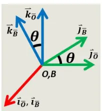
Figure 2.2 Rotation of the body fixed reference frame. . . 10

Figure 2.3 Free body diagram of the Tumbleweed rover. . . 19

Figure 2.4 Validation of the dynamic model. . . 25

Figure 2.5 Effect of changing the diameter of the rover on Earth. . . 28

Figure 2.6 Effect of changing the diameter of the rover on Mars. . . 28

Figure 2.7 Effect of changing the drag coefficient of the rover on Earth. . . 29

Figure 2.8 Effect of changing the drag coefficient of the rover on Mars. . . 29

Figure 2.9 Effect of changing the mass of the rover on Earth. . . 30

Figure 2.10 Effect of changing the mass of the rover on Mars. . . 30

Figure 2.11 Effect of changing the moving mass value of the rover on Earth. . . 31

Figure 2.12 Effect of changing the moving mass value of the rover on Mars. . . 32

Figure 3.1 Initial experimental setup. . . 39

Figure 3.2 Exploded view of the wind tunnel experimental setup. . . 40

Figure 3.3 Assembled wind tunnel experimental setup. . . 40

Figure 3.4 (a) Reference frames wind tunnel testing; (b) Wind tunnel test section. 41 Figure 3.5 Relative error contour graphs for dynamic pressure[5]. . . 43

Figure 3.6 Experimental setup validation result. . . 44

Figure 3.7 CD v s R e curve of the Box Kite. . . 45

Figure 3.8 Flow visualization of Box Kite. . . 45

Figure 4.1 (a) Tumbleweed Earth Demonstrator I[6]; (b) Scaled wind tunnel model of TEDI. . . 48

Figure 4.2 CD v s R e curve of TEDI. . . 48

Figure 4.3 (a) Tumbleweed Earth Demonstrator II[6]; (b) Scaled wind tunnel model of TEDII. . . 50

Figure 4.5 (a) Tumbleweed Earth Demonstrator III[6]; (b) Scaled wind tunnel model of TEDIII. . . 52 Figure 4.6 CD v s R e curve of TEDIII. . . 52 Figure 4.7 Comparison between theCD v s R e curves of the Box Kite, TEDI,

CHAPTER

1

INTRODUCTION

1.1

Overview of Mars Exploration

Mars represents the next great frontier for human exploration. Numerous robotic

space-crafts have visited the Red Planet after the development of spaceflight capability in the

mid-20th century. NASA’s Mars Pathfinder was a spacecraft that landed a base station with

a roving probe on Mars in 1997. It consisted of a lander and a small wheeled robotic rover

named Sojourner, which was the first rover to operate on the surface of Mars. NASA’s Mars

Exploration Rover Mission (MER), started in 2003, was a robotic space mission involving

ge-ology. The latest, most advanced and the only active rover on Mars, Curiosity was launched

in 2011 as part of NASA’s Mars Science Laboratory mission and it landed on Mars in 2012.

Figure 1.1: Distances driven by various rovers on Mars and the Moon[1].

The conventional wheeled rovers mentioned above are limited by their ability to operate

in a rugged terrain and have been able to cover relatively small portions of the Martian

surface. Their high cost and complexity has demanded a completely new approach to be

1.2

Overview of Wind-Driven Spherical Rovers

Jacques Blamont of JPL and the University of Paris conceived the first documented Mars

wind-blown ball in 1977. These proposed balls could be powered by the wind or could

be powered and steered by an inner drive mechanism [2]. Ten years later, in 1987, the

University of Arizona fabricated a large cylindrical device that was 4 m high by 5 m wide,

and had a mass of 500 kg. Although pneumatically driven this Mars ball was not a truly

wind driven rover[2].

In 1995, Jack Jones, et al, of JPL conceived of a large wind-blown ball for Mars that could

also be driven and steered by means of a motorized mass hanging beneath the rolling axis

of the ball. Jones then went on to develop a three-wheeled inflatable rover. In 2000, Jones

was testing this rover in a windy sand dune area in California’s Mojave Desert when one of

the wheels broke off and took off over the sand dunes. The 1.5 m diameter ball was able to

climb steep slopes, over large boulders, and through the jagged brush without hesitation.

This seemingly unlucky incident produced a rather lucky discovery and was the inspiration

for the current Tumbleweed rover. The University of Southern California, under contract to

JPL, confirmed that a 6 m diameter 20 kg inflatable Tumbleweed was capable of climbing

over large 1 m rocks and up 20° hills with moderately strong Martian seasonal winds of 20

m/s.

Numerous other researchers have also suggested spherical rovers. Almost all of them

have found the need to impart a certain degree of controllability to the rover through an

external driving mechanism but have faced problems. For example, the mass and power

requirements of the University of Arizona "Mars Ball" proved too large for realistic Mars

applications. The motorized concept used for the wind-blown Mars ball by Jack Jones, et

al, was abandoned when it was realized that the ball could inherently generate very little

(a) (b)

Figure 1.2: (a) The University of Arizona "Mars Ball"[2]; (b) J.Jones Inflatable Tricycle Rover[2].

Several deployments have been made with inflatable "Tumbleweeds" to some of the most

trying conditions on planet Earth including a 130 kilometer, wind-driven trek across

Antarc-tica.

(a) (b)

Figure 1.3: (a) A.Behar, Tumbleweed release at Amundsen-Scott South Pole station[2]; (b)

1.3

Overview of the Mars Tumbleweed Rover

The Langley Tumbleweed rover development started when it was observed that the Pathfinder

lander traveled further bouncing and rolling on it’s airbags in those few moments at landing

than the Soujourner rover traveled during it’s entire 90 sol mission. The Langley

Tumble-weed philosophy employed biomimetic theories in the design stages, primarily that nature,

being a highly efficient non-linear optimizer, has already pushed the development of the

desired characteristics in the Tumbleweed plants.

The Tumbleweed designs must have a mass less than 20 kg for a 6 meter diameter, for

the thin Martian air to provide sufficient aerodynamic force for sustained motion through

a Mars rock field. These calculations are based on the aerodynamic drag coefficient of a

smooth sphere. Wind tunnel tests performed at the Langley Basic Aerodynamic Research

Tunnel (BART) were used to quantify the drag characteristics of the various Tumbleweed

designs. Several initial concepts tested at Langley included the Tumblecup, Dandelion and

Box Kite. Wind tunnel tests have shown these designs to have a larger drag coefficient than

the sphere for the expected flow conditions.

A Mars Tumbleweed rover would therefore have to be extremely lightweight and equipped

with lightweight low-power instruments. If the Tumbleweed rover design could be kept

simple and in-expensive, it would allow relatively large numbers to be deployed for regional

or perhaps global coverage of the Martian surface, gathering scientific data to compliment

missions such as those carried out by the MERs. This concept is capable of overcoming the

drawbacks of traditional rovers but it has its own challenges and limitations. Directional

control and an effective aerodynamic design are a few of those design challenges posed

by the Mars Tumbleweed rover which have been addressed in this thesis. Also, the

aerody-namics of Tumbleweed Earth Demonstrators (TED) I, II and III has been studied which will

Thomas Estier and Moritz von Heimendahl developed a shape memory alloy (SMA)

actuated Tumbleweed-like windball while studying at the Swiss Federal Institute of

Tech-nology Lausanne (EPFL). The Texas Tech University Tumbleweed concepts were developed

as a senior mechanical engineering design class project.

Figure 1.4: NASA LaRC Tumbleweed rover concepts, from left to right Box-Kite, Dandelion,

CHAPTER

2

3D TUMBLEWEED ROVER DYNAMICS

Different forces like aerodynamic drag, weight, normal reaction, rolling resistance and

friction act on the Tumbleweed rover while it is in motion. The changing direction and

magnitude of these forces coupled with a moving center of gravity makes this an interesting

multibody system to study. Dynamic modeling helps us understand the effect of different

parameters on the acceleration, velocity and displacement of the Tumbleweed rover which

in turn determine its performance.

The first part of this chapter focuses on the development of the governing equations of

motion using the Newton Euler method. The obtained ordinary differential equations were

then solved numerically using MATLAB’s ode15s solver. At the end of this chapter, some

2.1

Reference Frames

2.1.1

Inertial Reference Frame

An inertial reference frame is defined as a frame whose origin does not accelerate and

whose axes do not rotate. Alternatively, it can be defined as a frame in which Newton’s

second law holds. In this case, ¯Ois defined as an Inertial reference frame.

¯

O = {O,i~_O¯,~j_O¯,k~_O¯}

2.1.2

Body Embedded Reference Frame

In this instance, ¯B is defined as the body embedded or body fixed reference frame. This reference frame is embedded or fixed at the geometric center of the rover and accelerates

as well as rotates along with it.

¯

B = {B,i~B¯,j~B¯,k~B¯}

2.1.3

Rotation Matrices

Figure 2.2: Rotation of the body fixed reference frame.

If the frame ¯Bis rotated about the axisi~B¯ by an angleθ, then to transform a vector expressed

in the ¯B frame to the ¯Oframe, we need to premultiply it by the rotation matrix[Rθ]X where,

[Rθ]X = 

   

1 0 0

0 c o s(θ) s i n(θ)

0 −s i n(θ) c o s(θ)

     (2.1)

θ is positive for counterclockwise rotation and negative for clockwise rotation. Similarly,

the rotation matrices for the Y and Z directions respectively are given by[Rφ]Y and[Rψ]Z where,

[Rφ]Y = 

   

c o s(φ) 0 ₋s i n(φ)

0 1 0

s i n(φ) 0 c o s(φ)

     (2.2)

[Rψ]Z = 

   

c o s(ψ) s i n(ψ) 0 −s i n(ψ) c o s(ψ) 0

0 0 1

2.1.4

Direction Cosine Matrix

If the ¯B frame is simultaneously rotated, first about the axis~iB¯ by an angleθ, second about

the axis ~jB¯ by an angle φ and third about the axisk~B¯ by an angleψ then the resultant

rotation matrix that we get is known as the direction cosine matrixB¯[C]O¯ _where,

¯

B_[C]O¯ _{= [Rψ]}

Z[Rφ]Y[Rθ]X (2.4)

If the sequence of rotation changes then the direction cosine matrix also changes

accord-ingly.

2.1.5

Angular Velocity

Now that the rotation matrices and direction cosine matrix have been defined, the angular

velocity of the ¯B frame relative to the ¯O frame,O¯_ω~B¯ _{can be defined as,} ¯

O_ω~B¯ ₌

where,

ωx = {0, 0, 1}

¯

B_[C]O¯O¯_[C˙]B¯

         0 1 0          (2.6)

ωy = {1, 0, 0}

¯

B_[C]O¯O¯_[C˙]B¯          0 0 1          (2.7)

ωz = {0, 1, 0}

¯

B_[

C]O¯O¯[C˙]B¯

         1 0 0          (2.8) ¯ O_[

C]B¯ = (B¯[C]O¯)T (2.9)

¯

O_{[ ˙}

C]B¯ = d d t(

¯

O_[

C]B¯) (2.10)

These definitions give the expressions forω_x,ω_y andω_z in terms ofθ_x,θ_y,θ_z, ˙θ_x, ˙θ_y and ˙

θz. These equations are then simultaneously solved for ˙θx, ˙θy and ˙θz in terms ofθx,θy,θz,

ωx,ωy andωz where,

˙

θx = (c o sθzωx−s i nθzωy)/c o sθy (2.11) ˙

θy = s i nθzωx+c o sθzωy (2.12) ˙

θz = ωz−s i nθy(c o sθzωx−s i nθzωy)/c o sθy (2.13)

It can be clearly seen that whenθy is an odd multiple ofπ/2, ˙θxgoes to∞and ˙θz goes to −∞which is not possible. Therefore to overcome this problem with Euler angles, Euler

2.1.6

Euler Parameters

The Euler parameters are denoted byq0,q1,q2andq3and are given by,

q0 = c o s(φ2)

q1 = axs i n(φ2)

q2 = ays i n(φ2)

q3 = azs i n(φ2)

(2.14)

wherea*={axi~O¯+ayj~O¯+azk~O¯}is assumed to be a unit vector. If *

a is imagined to be welded to the frame ¯B thenφis the angle through whicha*is rotated to obtain the final orientation of ¯B. The direction cosine matrixB¯_[C]O¯_{, in case of Euler parameters is given by,}

¯

B_[

C]O¯ =

     q2 0 +q

2 1 −q

2 2−q

2

3 2(q1q2+q0q3) 2(q1q3−q0q2)

2(q1q2−q0q3) q02−q 2 1 +q

2 2−q

2

3 2(q2q3+q0q1)

2(q1q3+q0q2) 2(q2q3−q0q1) q0−q12−q 2 2+q

2 3      (2.15)

and using the definitions mentioned in this chapter, it can be shown that,

               ˙ q0 ˙ q1 ˙ q2 ˙ q3                =1 2        

0 ₋ω_{x −}ω_{y −}ω_z

ωx 0 ωz −ωy

ωy −ωz 0 ωx

The normalization of Euler parameters is carried out using the method described by Fossen

[7]which is given below. The value ofγwas assumed to be 20 for the purposes of simulation.

               ˙ q0 ˙ q1 ˙ q2 ˙ q3                =1 2        

0 ₋ωx −ωy −ωz

ωx 0 ωz −ωy

ωy −ωz 0 ωx

ωz ωy −ωx 0                        q0 q1 q2 q3                + γ 2          1 ₋         q0 q1 q2 q3         T_        q0 q1 q2 q3                                 q0 q1 q2 q3                (2.17)

2.2

Governing Equations of Motion

As mentioned earlier, the governing equations of motion have been derived using the

Newton Euler method. Following relation is used to arrive on to the equations of motion.

X

~τB,s y s =

¯

O

d d t (

¯

O

Oh~B,s y s) +

¯

O_v~

B_/ O×M

¯

O_v~

C M_/

O (2.18)

Since, point B is neither the center of mass of the system nor a fixed point therefore, the

summation of the external torque about point B, acting on the system is equal to the rate

of change of the angular momentum about point B, of the system plus a correction term.

The LHS and RHS of Equation 2.18 must be expressed in the same reference frame for

equality to hold true and therefore all the quantities involved in the Equation 2.18 have

been expressed in the ¯B reference frame.

2.2.1

Forces and Torques Acting on the System

In this part of the chapter, mathematical expressions for the different forces acting on the

Tumbleweed rover as well as the torque due to them are developed.

Aerodynamic drag (F*D)

is a boundary layer and therefore a gradient. Wind speed at the ground is exactly zero.

But, it is assumed that the resultant aerodynamic drag acts at the geometric center of the

Tumbleweed rover and thus does not produce any torque about it.

*

FD = CD1/2ρ|

*

v∞|S

*

v∞(N) (2.19)

where,

CD = drag coefficient of the Tumbleweed rover

ρ = density of air(kg/m3) *

v∞ =relative wind velocity(m/s) = w* − O¯v~B_/

O (2.20)

S = area(m2) {F*D}B¯ =

¯

B_[

C]O¯· {F*D}_O¯ (2.21)

*

τa e r o d y n a m i c d r a g,B = 0 (2.22) Weight (F*g)

The direction of this force remains constant with time. The point of application of this force

continuously changes as weight acts at the center of gravity (cg) of the system and therefore

even the torque due to it keeps on changing depending on the location of the cg relative to

the geometric center.

*

where,

M = total mass of the Tumbleweed Rover(kg)

g = acceleration due to gravity(m/s2) {F*g}_B¯ =

¯

B_[

C]O¯ · {F*g}_O¯ (2.24)

*

τw e i g h t,B = r~C M_/ B ×

*

Fg (N −m) (2.25)

Normal reaction (F*N)

Normal reaction acts perpendicular to the surface of contact. Since only the rolling/sliding

motion of the Tumbleweed rover on a flat surface is considered here, the line of action

of normal reaction passes through the geometric center of the rover and thus does not

produce any torque about it.

X*

Fz = M azB¯k~O¯

*

FN − M gk~O¯ + FD zO¯k~O¯ = M azB¯k~O¯ *

FN = M azB¯k~O¯ + M gk~O¯ − FD zO¯k~O¯ (2.26) {F*N}B¯ =

¯

B_[

C]O¯ · {F*N}_O¯ (2.27)

*

τn o r m a l r e a c t i o n,B = 0 (2.28) Rolling resistance (f*r r)

Rolling resistance acts in a direction opposite to the motion of the body. It is assumed that

the rolling resistance acts at the geometric center of the Tumbleweed rover and thus even

this force does not produce any torque about point B.

*

fr r = −Cr r| *

FN|

¯

O_v~

B_/ O

|O¯_v~_B

/O|

where,

Cr r = coefficient of rolling resistance {f*r r}B¯ =

¯

B_[C]O¯

· {f*r r}O¯ (2.30)

*

τr o l l i n g r e s i s t a n c e,B = 0 (2.31) Friction (*f)

The direction of friction is such that it opposes any kind of relative motion between the

surfaces in contact. This means that it will assist rolling because in rolling the point of

contact is at rest. But, this holds true as long as the magnitude of friction required does not

exceedµs| *

FN|(µs- coefficient of static friction) after which the ground cannot provide more reaction force and the rover will start sliding. If the rover is rolling i.e._|*f | ≤ µs|

*

FN|then, According to the Newton’s second law,

X

~

Fe x t = M

¯

O_a~

C M_/ O

*

FD + *

Fg + *

FN + *

fr r + *

f = MO¯a~C M_/ O

*

f = MO¯a~C M_/ O −

*

FD − *

Fg − *

FN − *

fr r (2.32) *

τf r i c t i o n,B = r~P_/ B ×

*

f (2.33)

Using the second order transport theorem we get,

¯

O_a~

C M_/ O =

¯

O_a~

B_/ O +

¯

B_a~

C M_/ B + 2

¯

O_ω~B¯

×B¯ v~C M_/ B +

¯

O_~αB¯

×r~C M_/ B +

¯

O_ω~B¯

×O¯ ω~B¯×r~C M_/

B (2.34)

For the rolling condition to be satisfied,

¯

O_a~

B_/ O =

¯

O_~αB¯

×r~P_/

where,

~

rP_/

B =position vector of the point of contact i.e. pt P

relative to the geometric center i.e. pt B

= −Rk~O¯ (2.36)

{r~P_/ B}B¯ =

¯

B_[C]O¯ · {r~P_/

B}O¯ (2.37)

If the rover starts sliding then,

*

f = −µk| *

FN|

¯

O_v~

P_/O

|O¯_v~_P

/O|

(2.38)

where,

µk = coefficient of kinetic friction

¯

O_~

vP_/O = velocity of the point of contact

= _O¯

~

vB_/ O +

¯

O_ω~B¯ ×r~P_/

B (2.39)

{O¯v~B_/ O}B¯ =

¯

B_[C]O¯

· {O¯v~B_/

O}O¯ (2.40)

In such a situation, friction force is known andO¯_a~

C M_/

O is determined using the following

relation,

¯

O_a~

C M_/O =

*

FD + *

Fg + *

FN + *

f

M (2.41)

After findingO¯_a~

C M_/ O,

¯

O_a~

B_/

Figure 2.3: Free body diagram of the Tumbleweed rover.

Adding Equations 2.22, 2.25, 2.28, 2.31 and 2.33 we get the left hand side of Equation

2.18

X

~τB,s y s = r~C M_/B ×

*

Fg + r~P_/B×

*

f (2.42)

2.2.2

Angular Momentum of the System

This subsection of the chapter focuses on the development of the right hand side of the

Equation 2.18. The angular momentum about point B, of the system is given by,

¯

O

Oh~B,s y s =

¯

O

Oh~B,c h a s s i s +

¯

O

Oh~B,m a s s e s (2.43)

¯

O

d d t (

¯

O

Oh~B,s y s) =

¯

O

d d t(

¯

O

Oh~B,c h a s s i s) +

¯

O

d d t(

¯

O

Since, B=CM and also the frame ¯B forms the set of principal body axes for the chassis therefore,

¯

O

Oh~B,c h a s s i s = I˜B·

¯

O_ω~B¯ _(2.45)

where,

[_I˜_{B]B¯ =moment of inertia tensor of the chassis about point B(kg−m}2₎

=      ¯ B_I

x x/B 0 0 0 B¯Iy y/B 0 0 0 B¯Iz z/B

     (2.46)

Using the first order transport theorem we get,

¯ O d d t ¯ O

Oh~B,c h a s s i s=

¯ B d d t ¯ O

Oh~B,c h a s s i s+

¯

O_ω~B¯

×OO¯h~B,c h a s s i s = I˜B·

¯

O_~αB¯ ₊ ¯

O_ω~B¯

×(I˜B·

¯

O_ω~B¯₎

(2.47)

Now, by the definition of angular momentum,

¯

O

Oh~B,m a s s e s = n X

i=1

~

rmi_/B×m_iO¯v~mi_/O (2.48)

where,

n = number of moving masses

¯

O _d

d t

¯

O

Oh~B,m a s s e s = n X

i=1

mi (

¯

O _d

d t r~mi/B ×

¯

O_v~

mi_/O + r~mi_/B ×

¯ O d d t ¯ O ~

vmi_/O)

=

n X

i=1

mi (

¯

O_~

vmi_/B ×O¯ v~B_/

O + r~mi/B ×

¯

O _~

ami_/O) (2.49)

Using the second order transport theorem we get,

¯

O _~

ami_/O = O¯a~B_/ O +

¯

B_~

ami_/B + 2O¯ω~B¯×B¯ v~mi_/B + O¯~αB¯×r~mi_/B + O¯ω~B¯ ×O¯ ω~B¯×r~mi_/B (2.50)

Substituting the values from Equations 2.47 and 2.49 in Equation 2.18 we get,

¯

O _d

d t(

¯

O

Oh~B,s y s) +

¯

O_v~

B_/ O×M

¯

O_v~

C M_/

O = I˜B·

¯

O_~αB¯ ₊ O¯_ω~B¯ ×(I˜B·

¯

O_ω~B¯_{) +} n

X

i=1

mir~mi_/B ×

¯

O_a~

mi_/O (2.51)

Equations 2.42 and 2.51 are equated and solved forO¯~αB¯ where,

¯

O_~αB¯ _{= ω˙}

xB¯i~B¯ + ω˙yB¯j~B¯ + ω˙zB¯k~B¯ (2.52)

2.3

Solving the Equations of Motion

The Newton Euler equations of motion are ordinary differential equations and were solved

numerically using MATLAB’s ode15s solver.The equations thus obtained had to be

con-verted into a system of first order equations as the solver can only solve first order ode’s.

2.3.1

State Space Vector

The state space vector contains the variables that the ode solver computes and returns as

state space vector after each time step. In this instance, the state space vector contains

the x, y and z components of{r~m_1/

B}B¯,{r~m2/_B}_B¯,{r~m3/_B}_B¯,{r~m4/_B}_B¯,{r~m5/_B}_B¯,{r~m6/_B}_B¯,{r~C M_/ B}B¯, {B¯_v~

m_1/ B}B¯,{

¯

B_v~

m_2/ B}B¯,{

¯

B_v~

m3_/B}_B¯,{

¯

B_v~

m_4/ B}B¯,{

¯

B_v~

m5_/B}_B¯,{

¯

B_v~

m6_/B}_B¯ and{

¯

B_v~

C M_/

B}B¯. Additionally, it also consists of the Euler parametersq0, q1, q2, q3and the x, y and z components of

¯

O_ω~B¯_,

{r~B_/ O}O¯,{

¯

O_v~

B_/

O}O¯,{r~O/C M}O¯ and{

¯

O_v~

C M_/

O}O¯. As massm1can only move along+~iB¯, its position relative to the the geometric center i.e. point B is given by,

{r~m1/_B}_B¯ =

         r1 0 0          (2.53)

The position vector for massesm2,m3,m4,m5andm6can be defined in a similar way. All

the masses are constrained to move between an outermost radial positionrm a x and an innermost radial positionrm i n. Now, the position of the center of mass relative to point B can be given by,

~

rC M_/ B =

m1r~m1/_B+m₂r~m2/_B+m₃r~m3/_B +m₄r~m4/_B+m₅r~m5/_B+m₆r~m6/_B

M (2.54)

Once the position of massm1has been defined, its velocity can be defined as, ¯

B_~

vm1/_B =

¯

B

d

d tr~m1/B (2.55)

{B¯v~m1/_B}_B¯=

The velocity vector of other moving masses can be defined in a similar manner and the

velocity of the center of mass relative to point B is given by,

¯

B_v~

C M_/ B =

mB¯

1 v~m1/_B + m

¯

B

2v~m2/_B + m

¯

B

3v~m3/_B + m

¯

B

4v~m4/_B + m

¯

B

5v~m1/_B + m

¯

B

6 v~m1/_B

M (2.57)

2.3.2

ODE Function

The ode solver evaluates the updated state space vector after every time step using the ode

function. The ode function contains the first derivative of the variables present in the state

space vector. Initially, it is assumed that the rover is rolling and the Equations 2.42 and 2.51

are numerically solved for ˙ωxB¯, ˙ωyB¯, ˙ωzB¯. These values are then used to get the magnitude

of friction force which is then checked for the no slip condition i.e._|*f| ≤ µs| *

FN|. If this condition is satisfied then the assumption made is correct otherwise the rover is sliding

and the corresponding equations for sliding are used.

2.4

Simulation Results

Simulations can predict the actual behaviour of a system before it is built and put to test

in the real world. The higher the accuracy of the model used for simulation, the better

it will imitate the real world performance of the system. Simulations can also lower the

experimental costs required, in some cases even eliminate it and guide in taking major

design decisions before the final product is made.

Results from a few test cases are presented below where the Tumbleweed rover is

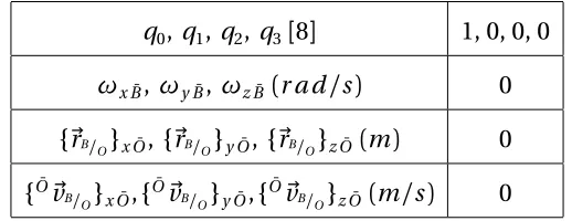
Table 2.1: Initial conditions used for all the simulations

q0, q1, q2, q3[8] 1, 0, 0, 0

ωxB¯, ωyB¯, ωzB¯ (r a d/s) 0

{r~B_/

O}xO¯, {r~B/O}yO¯, {r~B/O}zO¯ (m) 0

{O¯_v~

B_/ O}xO¯,{

¯

O_v~

B_/ O}yO¯,{

¯

O_v~

B_/

O}zO¯ (m/s) 0

2.4.1

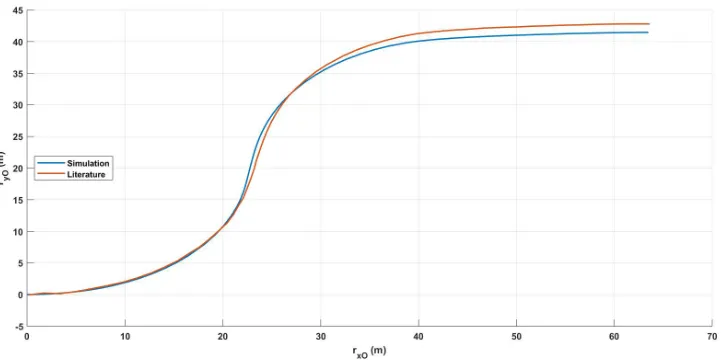
Validation of the Dynamic Model

For the purpose of validation, the simulation result from this dynamic model is compared

to the simulation result presented in[9], where the Tumbleweed rover is subjected to the

following wind distribution,

wx = 7c o s(18t), wy = 7s i n(18t), wz = 0}f o r 0 ≤ t ≤10

wx = 7c o s(18t), wy = 0, wz = 0}f o r 10 < t ≤15

wx = 0, wy = 0, wz = 0}f o r 15 < t ≤ 40

wherewx,wy andwz are winds alongi~O¯, ~jO¯ andk~O¯ respectively and angle is measured in degrees. Apart from the initial conditions given in Table 2.1, other simulation parameters

used are given in Table 2.2. This simulation shows the effects of changing wind on the

Table 2.2: Physical conditions and properties used for the validation case

ρ(k g/m3_{) 1.2}

CD 0.5

g (m/s2_{) 9.81}

µs 0.1

µk 0.08

Cr r 0.1

M (k g) 20

R(m) 5

¯

B_I x x/B,

¯

B_I y y/B,

¯

B_I

z z/B (k g −m2) 200

2.4.2

Effect of Varying Different Parameters on the Performance of the

Tumbleweed Rover

The outcomes on changing the various parameters of the Tumbleweed rover were assessed.

The rover was considered as a hollow sphere for the purpose of simulation. Table 2.3

con-tains the physical conditions, properties and initial conditions used for all the simulations.

Only one parameter was changed at a time, keeping all the other parameters constant. This

isolated the effect of that specific parameter on the directional control of the rover. The

simulations were carried out for atmospheric conditions on Earth as well as on Mars. The

air density on Mars is about 80 times lesser than that on Earth while the gravity on Mars is

approximately one third the Earth’s gravity. This makes it relatively more difficult to derive

Table 2.3: Physical conditions, properties and initial conditions for all the simulations

m1, m2, m3, m4, m5, m6(k g) 0

ρ(k g/m3_{) 1.225 (Earth)}

0.0155 (Mars)

CD 0.5

g (m/s2_{) 9.81 (Earth)}

3.72 (Mars)

µs 0.5

µk 0.4

Cr r 0.06

M (k g) 20

R (m) 0.75 (Earth)

3 (Mars)

¯

B_I x x/B,

¯

B_I y y/B,

¯

B_I

z z/B (k g−m2) 25M R 2

rm a x (m) 0.55 (Earth) 2.2 (Mars)

rm i n (m) 0.25 (Earth) 1 (Mars)

r1, r3, r5(m) 0.4

r2, r4, r6(m) -0.4

v1, v3, v5(m/s) 0

v2, v4, v6(m/s) 0

Figures 2.5 and 2.6 depict that the rover reacts faster to the wind variations as its diameter

increases. The bigger diameter rovers cover the same amount of distance in a shorter period

of time. Aerodynamic drag which is the driving force is directly proportional to the square

of the diameter of the rover, so even a slight increase in the diameter increases the drag

effectiveness of increasing the diameter decreases as the diameter increases.

Figure 2.5: Effect of changing the diameter of the rover on Earth.

Figure 2.6: Effect of changing the diameter of the rover on Mars.

coefficient as well that can be clearly seen in the Figures 2.7 and 2.8. Since the drag force is

only linearly proportional to the drag coefficient, the resulting trends are not as evident as

they were in case of an increase in the diameter.

Figure 2.7: Effect of changing the drag coefficient of the rover on Earth.

Rolling resistance decreases linearly with a decrease in the mass of the rover. Therefore, it

becomes easier for the rover to move as its mass decreases which is visible in the Figures

2.9 and 2.10. Also, the effectiveness of decreasing the mass increases as the mass decreases.

Figure 2.9: Effect of changing the mass of the rover on Earth.

Figures 2.11 and 2.12 demonstrate the ability of the moving masses to control the motion

of the Tumbleweed rover. For this simulation, massesm1,m3andm5begin moving toward

their outermost radial position at t=7.5 seconds, simultaneously massesm2,m4andm6

move toward their innermost radial position. Once the masses reach their extreme position,

they stay there till t=15 seconds, after which they start moving toward their opposite end at

t=15 seconds. Again, the masses are actuated at t=22.5 seconds to move to their opposite

ends, after which they stay there till the end of the simulation. The value ofCr r was assumed to be 0.002 for this simulation. These results illustrate the capabilities of the Tumbleweed

rover to negotiate the Martian terrain in presence of an optimum control scheme for the

actuation of masses.

CHAPTER

3

AERODYNAMICS OF THE BOX KITE

As Tumbleweed rover is a wind driven rover and primarily relies on aerodynamic drag for

propulsion therefore, it is important to study and understand its aerodynamics. Previously,

a comparison of different ideas for the Tumbleweed rover, like the Box Kite, Dandelion,

Tumblecup and Wedges has been done by the researchers at NASA and the Box Kite seemed

to have shown the most promising characteristics[3]and[4]. An aerodynamic analysis of

the Box Kite gives an idea of its drag coefficient and flow over it which in turn help determine

the force acting on the Tumbleweed rover.

This chapter aims to create a better understanding of the aerodynamics of the Box

Kite over a range of Reynolds numbers. It explains the calculation of the drag coefficient

presented in this chapter.

3.1

Wind Tunnel Testing

Wind tunnel testing being the more accurate and less time consuming method over

com-putational fluid dynamics (CFD), is chosen as the first step in the research process here.

3.1.1

Reynolds Number

Reynolds number is the ratio of inertia force to viscous force and is given by,

R ed =

I n e r t i a F o r c e V i s c o u s F o r c e =

ρ∞v∞d

µ∞

= v∞d

ν∞

(3.1)

where,

ρ∞ = freestream density(kg/m3)

v_∞ = freestream velocity(m/s)

d = diameter(m)

µ∞ = freestream dynamic viscosity(kg/ms)

ν∞ = freestream kinematic viscosity(m2/s)

= µ∞

Table 3.1: Air properties on Earth and Mars

ρ∞(k g/m3) µ∞(k g/m s) ν∞(m2/s)

Earth 1.225 1.7885_×10−5 _1.46×10−5

Mars 0.0155 1.24_×10−5 _8×10−4

The data available shows the freestream velocity on Mars to be 2 to 7 m/s (summer),

5 to 10 m/s (fall) and 17 to 30 m/s (dust storm)[10]. Prior studies have shown that the

Tumbleweed rover needs to be 4 to 6 m in diameter with a mass between 10 to 20 kg in order

for it to achieve mobility through the Martian environment[4]. With these parameters, a 6

m Tumbleweed rover in wind speeds ranging from 2 to 30 m/s will be at Reynolds numbers

ranging from 15,000 to 225,000.

3.1.2

Flow Similarity

Flow similarity is what allows the testing of scaled models in wind and water tunnels. If the

two flows are dynamically similar, then,

i. the streamline patterns are geometrically similar,

ii. the distributions of_vv

∞,

p p∞,

T

T∞ throughout the flow-field are the same when plotted

against common non-dimensional coordinates and

iii. the force and moment coefficients are the same.

The criteria for dynamically similar flows are that

i. the bodies and any solid boundaries must be geometrically similar for the two flows

ii. the similarity parameters must be the same for both the flows.

The two most common similarity parameters in aerodynamics are Reynolds number (Re)

and Mach number(M). In this case, only the Reynolds number of the actual Tumbleweed

rover is matched to the Reynolds number of the scaled wind tunnel model.

3.1.3

Wind Tunnel Model

Ideally, from the flow similarity condition,

(R e)s c a l e d w i n d t u n n e l m o d e l = (R e)a c t u a l T u m b l e w e e d r o v e r (3.2)

But, in reality a turbulence factor (TF) needs to be taken into account and is defined as,

T F = (R e)c r i t i c a l o f a s p h e r e i n a n o n t u r b u l e n t a i r s t r e a m

(R e)c r i t i c a l i n t h e t u n n e l

(3.3)

= 1.2515(for the NCSU subsonic wind tunnel)

Now,

T F ×(R e)s c a l e d w i n d t u n n e l m o d e l = (R e)a c t u a l T u m b l e w e e d r o v e r (3.4)

For a fixed diameter, the Reynolds number can be varied by varying the freestream velocity.

Keeping in mind the free stream velocity, blockage ratio and the load cell resolution,

diam-eter of the wind tunnel model was chosen to be 73 mm at first but was later changed to 80

mm for a reason explained later.

The wind tunnel model was 3D printed using the Fused Deposition Modeling (FDM)

technique on a Stratasys F370 3D printer. The material used was ABS plastic and the 3D

surface finish.

3.1.4

Dynamic Pressure

The freestream velocity is changed by changing the dynamic pressure and cannot be directly

controlled. The dynamic pressure is given by,

q = 1

2ρv

2

∞(P a) (3.5)

The values of freestream velocity obtained from Equation 3.3 are substituted in the Equation

3.5 to get the range of dynamic pressures. It turns out that the freestream velocity varies

from 2.15 m/s to 32.30 m/s and the corresponding dynamic pressure varies from 0.06 psf

to 13.42 psf.

3.1.5

Wind Tunnel

North Carolina State University’s subsonic wind tunnel is a closed circuit tunnel powered by

a variable speed 150 hp electric motor and is capable of speeds upto 100 mph. Test section

dimensions of the tunnel are 33”h i g h×43”w i d e×48”l o n g. The tunnel blockage ratio is defined as,

B l o c k a g e R a t i o (%) = f r o n t a l a r e a o f t h e m o d e l

c r o s s s e c t i o n a l a r e a o f t h e t e s t s e c t i o n ×100 (3.6)

= 0.55%

Since the blockage ratio is less than 1%, therefore no blockage correction needs to be taken

3.1.6

Force

/

Moment Balance

An ATI Gamma IP65 six-axis load cell was used as the force/moment Balance for the

mea-surement of forces and torques.

Table 3.2: Load cell specifications

Fx,Fy Fz Tx,Ty Tz

SENSING RANGES 130 N 400 N 10 Nm 10 Nm

RESOLUTION 1/40 N 1/20 N 1/800 Nm 1/800 Nm

3.1.7

Experimental Setup

Figure 3.1 illustrates the experimental setup used at first but this setup led to erroneous

readings because the wake of a sphere has effects upto six times its diameter, which was

later discovered[11]. Therefore, such an arrangement would require a really long length of

the sting (upto eight times the sphere diameter) which was seemingly not a good idea and

thus a new setup had to be designed and manufactured. Since the drag of bluff bodies is

dominated by pressure drag, it had to be ensured that the flow past the sphere is clean and

Figure 3.1: Initial experimental setup.

Figure 3.2 shows the different components of the new setup. The beta plate can be moved

along the slots on the alpha plate while the load cell mount plate can be moved along the

slots on the beta plate to test the model at different combinations of angles of attack (α)

and side slip angles (β). The directions of rotation are shown using black arrows in the

Figure 3.2. In both these cases, angle can be varied from 0° to 45° (0°≤α,β≤45°). The sting

female part is connected to the sting male part using a threaded joint and the model is

press fitted on to the sting female part. Apart from these all other connections are bolted.

Lastly, the base plate is bolted to a stool as shown in Figure 3.3.

The alpha plates, beta plate, load cell mount plate and base plate were water jet cut while

the sting male and female parts were machined to the required dimensions.To reduce the

material wastage and to increase the functionality of the setup, the sting was not machined

Figure 3.2: Exploded view of the wind tunnel experimental setup.

(a) (b)

3.1.8

Experiment Procedure

The data was acquired using LabVIEW. After assembling the experimental setup, the load

cell was biased to negate the effect of initial loads acting on it. Once the load cell was biased,

the tunnel was switched on and the dynamic pressure was reduced to 0.06 psf. The tunnel

was then set at gradually increasing values of dynamic pressure starting at 0.06 psf going

up to 13.42 psf and at each of those predecided values the data was collected for about 30

seconds. Average values over a span of 30 seconds were considered. The motor was ran on

low speed for dynamic pressures below 5 psf, medium speed for dynamic pressures in the

range 5-10 psf and high speed for dynamic pressures above 10 psf. The load cell records

the values ofFx, Fy, Fz (i n l b f), Tx, Ty, Tz (i n l b f −i n)at a frequency of 10 khz while the wind tunnel records the values ofq (p s f), q (P a), T (°F), T (°C), ρ(k g/m3_{), v}

∞(m/s)at

a frequency of 1khz.

(a) (b)

Figure 3.4: (a) Reference frames wind tunnel testing; (b) Wind tunnel test section.

frame ¯B. Next, the forces due to the sting were recorded at those same values of dynamic pressure and then subtracted from the forces recorded by the load cell when the model was

mounted on the sting. This gave the forces acting on the model in the frame ¯B which were then converted to the frame ¯O using the direction cosine matrix (refer 2.1.4).

{FD}_O¯ = O¯[C]B¯· {FD}B¯ (3.7)

where,

¯

O_[

C]B¯ = (B¯[C]O¯)T (3.8)

¯

B_[C]O¯ _{= [Rβ]}

Z[Rα]X (3.9)

{FD}_B¯ = {FD (m o d e l+s t i n g)}B¯ − {FD(s t i n g)}B¯ (3.10)

The force coefficients are then obtained from the forces using the following relation,

        

CD x

CD y

CD z          = 1 q S         

FD xO¯

FD yO¯

FD zO¯          (3.11)

3.2

Wind Tunnel Results

Like always, the first step was to validate the experimental setup only after which the Box

Kite was tested in the tunnel. Figure 3.5 depicts the relative error in the dynamic pressure

across the tunnel cross section at 0.5 psf and 1.25 psf. The relative error reduces considerably

as q increases from 0.5 psf to 1.25 psf. Although the error percentages are overestimated

according to the author, they capture the right trend that the quality of the flow near the

unsteadiness of the tunnel at low values of q, even though the measurements were taken

from 0.06 psf upto 13.42 psf, only the measurements taken after 1.2 psf are considered.

(a) (b)

Figure 3.5: Relative error contour graphs for dynamic pressure[5].

3.2.1

Experimental Setup Validation

The experimental setup was validated through a sphere test. Drag coefficient of a sphere of

the same diameter was found out over the same range of Reynolds numbers as the Box Kite

and compared with the results presented in the literature.CD x was almost zero throughout the range of Reynolds numbers as expected. The values ofCD y are a bit on the higher side as compared to the values in the literature depicted in Figure 3.6[12]. Asymmetrical flow

around the sphere due to the sting was the reason for a non-zeroCD z. The wake of the sting created a low pressure region below the sphere which caused a force on the sphere

along the -k~_O¯ direction. It was seen that the magnitude ofC_{D z} decreased as the model

diameter was increased from 73 mm to 80 mm. A dummy sting can eliminate this force,

Figure 3.6: Experimental setup validation result.

3.2.2

Wind Tunnel Results of the Box Kite

The Box Kite behaved like three orthogonal circular flat plates in a flow, two of which were

aligned parallel and one was aligned perpendicular to the flow. Figure 3.7 shows a slight

drop in the drag coefficient of the Box Kite with increasing Reynolds numbers. A similar

Figure 3.7: CD v s R e curve of the Box Kite.

The flow visualization studies were done at a Reynolds number of 88,500. The Box Kite

exhibits flow dynamics similar to a flat plate perpendicular to the flow. Figure 3.8 depicts

the flow turning at nearly right angles as it is about to impact the plate and then turns to

escape the corner and continue downstream.

CHAPTER

4

AERODYNAMICS OF THE TUMBLEWEED

EARTH DEMONSTRATORS

The Box Kite as a structure cannot roll on the surface and needs an outer structure that

improves its rolling properties. This led to the development of the Tumbleweed Earth

Demonstrator (TED). A series of TEDs have been designed, constructed and tested by NCSU.

The design included, not only the outer structure, but the instrumentation, propulsion,

deployment, packaging and transport. The purpose of these TEDs was to emulate the

capabilities of Mars Tumbleweed in Earth’s atmospheric conditions.

TEDI, TEDII and TEDIII. The results from the wind tunnel tests of each of these TEDs have

been presented in this chapter.

4.1

Tumbleweed Earth Demonstrator I

NCSU’s first TED was designed and constructed during the 2002-03 academic year. It

became known as the TEDI and was the first in a succession of TEDs. The TEDI was

con-structed as a one-third scale (2 meter diameter) prototype of the Tumbleweed rover. The

TEDI had a rigid outer structure, with orthogonal sails to create drag and therefore propel

the TED. It had a fixed instrument core in the center of the structure and solar panels on

the sails.

The inner structure of the TEDI had a basic Box Kite configuration. It consisted of

three, three inch diameter orthogonal hoops made of a carbon fiber/kevlar hybrid. The

hoops were covered in a flexible sail material with an instrument core located in the center.

Additional hoops without sail material, were added to assist the rolling properties.Figure

(a) (b)

Figure 4.1: (a) Tumbleweed Earth Demonstrator I[6]; (b) Scaled wind tunnel model of

TEDI.

4.2

Tumbleweed Earth Demonstrator II

After testing of the TEDI, it was evident that a two meter diameter did not provide sufficient

sail area to create enough drag to propel the TED. The next generation of TEDs needed

to be lighter weight and have a larger sail area. This new design became known as TEDII.

The TEDII had a diameter of three meters which after testing proved to be enough sail

area to propel the structure provided a large enough wind speed. TEDII’s design had also

been improved from the previous TEDI by adding a sail retraction and deployment system

(SRDS) and a gimbaled modular instrument system (MIS) with solar pannels on the upper

face.

The outer structure of the TEDII was made up of a 2-inch carbon fiber/kevlar hybrid

sleeve. The hybrid sleeve was chosen for its light weight, strength and durability. The

structure was composed of 24 main members, 2 hubs, and 1 center ring. The main members

were divided in two, attached to the hubs and connected to each and the center ring via

a 4-way joint. This joint was made of polyvinyl chloride(PVC) and the members were

attached using nylon bolts. The hubs were made of the same sleeve material used for the

main members. Each hub had 12 appendages, with 30 degrees separating each. The inner

structure consisted of six hollow aluminum struts that attach the double gimbal system

(DGS) to the outer structure. The completed TEDII, with sails, DGS and MIS is shown in

(a) (b)

Figure 4.3: (a) Tumbleweed Earth Demonstrator II[6]; (b) Scaled wind tunnel model of

TEDII.

4.3

Tumbleweed Earth Demonstrator III

Given TEDII’s increased size and weight the outer structure similar to TEDI, began to buckle

under rolling loads. A more rigid structure would be needed to preserve the spherical shape

and protect the gimbaled MIS inside. These requirements, again resulted in another

gener-ation called TEDIII. This TEDIII’s outer structure was made of PVC piping and provided

enough rigidity to exhibit a structured Mars Tumbleweed capabilities. The TEDIII also had

a new SRDS and a new MIS.

The main purpose of TEDIII was to improve upon the previous TED designs so testing

could be conducted. Stronger materials needed to be used to construct the outer structure

of the TED to withstand its own weight. Therefore the TEDIII outer structure was made of

one and one half inch schedule 40 PVC pipe, which allowed the TED to remain adequately

rigid. This, however, required a new hub design that was smaller and stronger. The new

hubs were made of ungalvanized steel, which were smaller in size but increased the weight.

Two side rings were also added to better distribute the dynamic stress applied on the outer

structure. These side rings were made of the same PVC pipe as the outer structure. The

new PVC structure was formed by bending the PVC pipe to the correct radius using a rig,

heating the pipe using boiling water and allowing it to cool while remaining in its deformed

shape. The main members were connected to the two hubs and the center and outer rings

were connected to the main members using 4-way connectors, inserts and velcro. Figure

(a) (b)

Figure 4.5: (a) Tumbleweed Earth Demonstrator III[6]; (b) Scaled wind tunnel model of

TEDIII.

4.4

Comparison between TEDI, TEDII and TEDIII

This section compares the drag coefficient of the Box Kite, TEDI, TEDII and TEDIII which

helps understand the effect of the outer structure on the drag coefficient of the internal

Box Kite. In the presence of an outer structure, a small fraction of the oncoming airstream

flows over the outer surface instead of being directly intercepted by the Box Kite plate. It

is the reason why all the TEDs have a drag coefficient lesser than that of the Box Kite at

the corresponding Reynolds number depicted in Figure 4.7. Greater is the surface area of

the outer structure, greater is the drop in the drag coefficient. Hence, TEDI has the lowest

while TEDII has the highest drag coefficient of the three TEDs. This argument is supported

through the flow visualization results presented in Figure 3.7.

Figure 4.7: Comparison between theCD v s R e curves of the Box Kite, TEDI, TEDII and